HW pandas

Instructions

Please use Python 3.6+ (never Python 2).

For other packages: Although I didn’t run all the tests, there will likely be no problem if you use decently recent versions of any packages used in the homework (any version released after 2017).

Here, we will learn how to code in pythonic way. Start solving the problems after running the code below:

import numpy as np
import pandas as pd
from matplotlib import pyplot as plt

plt.style.use('default')
np.random.seed(123)
data_str = '''jd_target,m_red,dm_red,serious
    2458403.9602,17.1008,0.0738,0
    2458403.9722,17.1255,0.0429,0
    2458403.9842,17.1770,0.0420,0
    2458403.9961,17.2755,0.0412,0
    2458404.0081,17.3114,0.0435,0
    2458404.0201,17.3947,0.0377,0
    2458404.0321,17.2879,0.0340,0
    2458404.0440,17.2120,0.0312,0
    2458404.0560,17.0571,0.0277,0
    2458404.0680,17.0799,0.0277,0
    2458404.0800,17.0958,0.0272,0
    2458404.0920,17.1262,0.0271,0
    2458404.1040,17.2231,0.0304,0
    2458404.1159,17.3279,0.0312,0
    2458404.1401,17.2705,0.0277,0
    2458404.1521,17.1999,0.0222,0
    2458404.1641,17.0976,0.0209,0
    2458404.1761,17.0944,0.0228,0
    2458404.1881,17.0537,0.0249,0
    2458404.2001,17.0836,0.0249,0
    2458404.2122,17.1790,0.0245,1
    2458404.2242,17.2610,0.0303,0
     '''

While answering the problems, follow these rules:

1. You should not import any other packages.

2. For each problem, I gave hints. It is also homework for you to search for those on Google.

Problems [40 points]

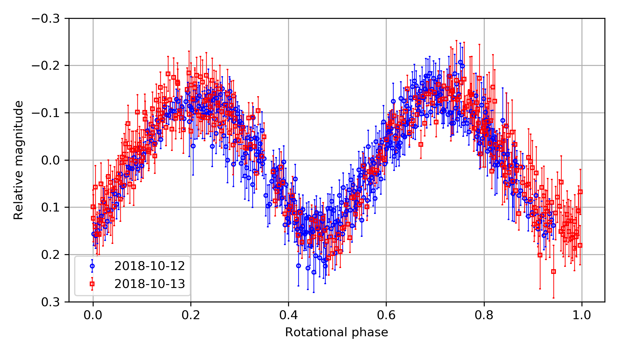
The data_str is the photometry result of an asteroid (155140) 2005 UD taken at the SNU Astronomical Observatory (SNUO or SAO) 1-m telescope. I selected only 22 data points out of 811 data points. jd_target is roughly the observation time in JD, m_red is the reduced magnitude (please regard it as the magnitude of the asteroid), dm_red is the error of it, and serious is 1 if the image had a serious problem, so it should not be used.

Reference

The results from this observation are published as Ishiguro, Bach, Geem et al. 2022, and the reduction/plotting codes are available via GitHub.

• Publication: Ishiguro M., Bach Y. P., Geem J., et al. (2022) MNRAS, 509, 4128

• ADS: 2022MNRAS.509.4128I

• DOI: 10.1093/mnras/stab3198

[2 points each]

You can fill in the >>FILLHERE<< parts in the Hints and use that to answer the questions. Or, you can just make your own answer, ignoring the Hints.

1. Make a DataFrame from data_str. Give it the name df.

   • Hint: pd.read_csv(pd.compat.StringIO(?))

2. Print the first 3 rows of the df.

   • Hint: use .head()

3. Print the last 3 rows of the df.

   • Hint: use .tail()

4. See df.describe(). What is the roughly estimated mean magnitude?

5. Print the latex code for the data to make a table.

   • Hint: use print(df.to_latex(index=False))

   • There are other conversions, to HTML, numpy, etc.

6. Check whether the unique elements of the column serious are 0 and 1.

   • Hint: use .unique() to the column.

7. To get an idea of how the data looks, plot the error-bar of m_red as a function of JD.

   • Hint: plt.errorbar(df["jd_target"], df["?"], df["dm_red"])

8. The error-bar of magnitude is not Gaussian, but the error-bar of flux is nearly Gaussian. In usual photometry, what we get is the flux error, but we only present the magnitude error, which is calculated (estimated) from the flux error. From dm_red, recover the error-bar of the flux.

   • Hint: The flux error and magnitude error are related by dm = 2.5 / np.log(10) * dflux.

   • Hint: The inversion of the equation may give df["dflux"] = ? * df["dm_red"]

9. Actually, "dflux" column is useless. Remove this column.

   • Hint: Use .drop(columns=["dflux"], inplace=?).

   • The inplace option can either be True or False, depending on how you do it (if you can’t understand it, Google it!)

10. Make a mask to mask rows with serious==1. Name it mask_serious.

    • Hint: df["serious"]==1

11. Replace the dm_red of the masked row with NaN.

    • Hint: Use df.loc[mask, "dm_red"]

12. You found that, for some reason, the 3-th row is problematic. Replace "m_red" in this row with NaN.

    • Hint: Use df.loc[3, "m_red"] or df.iloc[3, 1].

13. Drop any row that contains any NaN values.

    • Hint: Use df.dropna(inplace=?)

14. If you see df, the index (leftmost column) is missing 3 and 20. Reset this such that it is consecutive integers of separation 1.

    • Hint: df.reset_index(inplace=?, drop=True)

15. From Ishiguro et al. 2019, it is found that the period of the asteroid is 0.218282 +/- 0.000092 days. Add a column called "phase".

    • Hint: Use df["jd_target"]%0.218282 / 0.218282

16. Make a column "first_half", and assign True if the phase is smaller than 0.5 and False otherwise.

    • Hint: df["first_half"] = df["phase"] < 0.5

17. Make a column "faint", and assign True if m_red is larger (fainter) than the mean calue, and False otherwise.

    • Hint: df["faint"] = df["m_red"] > df["m_red"].mean()

18. Make DataFrameGroupBy object based on the columns ["first_half", "faint"].

19. [4 points] Fill in the following code to plot a graph such that the marker is

    1. red when first_half==True and blue otherwise,

    2. empty inverse triangle ("v") when faint=True and filled triangle ("^") otherwise and the y-axis decreases as you go upward (lower 17.5, upper 17.0) because of it’s the magnitude.

    #        first  faint
    props = {(True, True): dict(marker="v", color="r", mfc="none"),
             (True, False): dict(marker="^", color="r"),
             (False, True): dict(marker="v", color="b", mfc="none"),
             (False, False): dict(marker="^", color="b")
            }
    
    fig, axs = plt.subplots(1, 1, figsize=(6, 4), sharex=False, sharey=False, gridspec_kw=None)
    
    for (first, faint), g in grouped:
        axs.errorbar(g["phase"], g["m_red"], yerr=g["dm_red"],
                     **props[(>>FILLHERE<<, >>FILLHERE<<)], ls='', ms=10)
    
    axs.set(ylim=(>>FILLHERE<<, 17),
            xlabel="Phase", ylabel="Reduced magnitude")
    axs.grid()
    plt.tight_layout()
    plt.show()
    

TIP

There are some occasions when it’s better to use for than the simple df["blahblah"] = df["col1"] * df["col2"], especially when complicated calculations are needed. In such cases, you can use

for i, row in df.iterrows():
    first_half = row["phase"] < 0.5
    df.at[i, "first_half"] = first_half

Things go well in this case with loc, but I used at.

• loc is slower, but you can access multiple locations.

• at is quicker, but you can access only one single location.

See here

The full light curve of this asteroid, from the 2-night observation at SNU, is like this: