1. Basics about FITS#
This part will teach you:
Read/write FITS files.
Crop (cutout) a small region of the FITS image.
The data we will use for the next few notes are from the Korean KMTNet, the observation of an asteorid (4179) Toutatis. The results are published as Bach, Ishiguro, Jin, et al. (2019) JKAS
# Ignore this cell if you encounter errors
%load_ext version_information
import time
now = time.strftime("%Y-%m-%d %H:%M:%S (%Z = GMT%z)")
print(f"This notebook was generated at {now} ")

vv = %version_information astropy, numpy, scipy, matplotlib, version_information
for i, pkg in enumerate(vv.packages):
    print(f"{i} {pkg[0]:10s} {pkg[1]:s}")
This notebook was generated at 2023-05-09 16:08:52 (KST = GMT+0900)
0 Python     3.10.10 64bit [Clang 14.0.6 ]
1 IPython    8.13.2
2 OS         macOS 13.1 arm64 arm 64bit
3 astropy    5.2.2
4 numpy      1.24.3
5 scipy      1.10.1
6 matplotlib 3.7.1
7 version_information 1.0.4
# %matplotlib notebook
from IPython.core.interactiveshell import InteractiveShell
from IPython import get_ipython
%config InlineBackend.figure_format = 'retina'
InteractiveShell.ast_node_interactivity = 'last_expr'
ipython = get_ipython()

from pathlib import Path
import numpy as np

from astropy.io import fits
from astropy.time import Time
from astropy import units as u
from astropy.nddata import CCDData

from matplotlib import pyplot as plt
from matplotlib import rcParams

import ysfitsutilpy as yfu
import ysphotutilpy as ypu

plt.style.use('default')
rcParams.update({'font.size':12})

import warnings
warnings.filterwarnings('ignore', category=UserWarning, append=True)

import _tool_visualization as vis

DATAPATH = Path('../../Tutorial_Data')
TMPDIR = Path('tmp')
TMPDIR.mkdir(exist_ok=True)
allfits = list(DATAPATH.glob("*p4179*.fits"))
allfits.sort()
print(f"Found {len(allfits)} fits files in {DATAPATH}.")
for _f in allfits:
    print(_f)
Found 7 fits files in ../../Tutorial_Data.
../../Tutorial_Data/20180413SAAO_p4179_010449.fits
../../Tutorial_Data/20180413SAAO_p4179_010451.fits
../../Tutorial_Data/20180413SAAO_p4179_010453.fits
../../Tutorial_Data/20180413SAAO_p4179_010455.fits
../../Tutorial_Data/20180413SAAO_p4179_010457.fits
../../Tutorial_Data/20180413SAAO_p4179_010459.fits
../../Tutorial_Data/20180413SAAO_p4179_010461.fits
1.1. astropy.fits#
You may have already learnt astropy.fits package from python preperation class. Here, I will review that and introduce a little bit more.
The official documentation of astropy is here. Among those, we will learn about astropy.io.fits module, which is one of the greatest tool to handle FITS format.
Some information of the terms: FITS : See this
- HDU
Header Data Unit. An HDU is composed of Primary header (optionally with data) and other header & data. The simplest one contains only the primary HDU.
- HDU List
python
listof the HDU objects- MEF
Multi-Extension FITS. In some cases, more than one such HDU is present in one FITS file. That is called the MEF. MEF is not recommended unless you are clearly aware of what you are doing.
- Header
Contains information about the image. The most standard keywords are here and others can be found at here. Few important ones are
OBJECT: The name of the targetDATE-OBS: The time when the exposure started (in UT). Mostly in the format ofYYYY-MM-DDTHH:mm:ssfollowing ISO 8601, e.g.,2019-01-02T13:01:01means it was taken on 2019 Jan 2nd, at 13:01:01. Sometimes (some observatories) only give YYYY-MM-DD or other unorthodox formats…EXPTIME: The exposure time in seconds.NAXIS1: The number of pixels along the axis 1 (which is the X axis). Same forNAXIS2.FILTER: Not a standard, but widely used to show the filter (e.g.,VorJohnson B, etc).
Some basic usages are as follows:
for fpath in allfits:
    hdul = fits.open(fpath)
    hdul.info()
Filename: ../../Tutorial_Data/20180413SAAO_p4179_010449.fits
No.    Name      Ver    Type      Cards   Dimensions   Format
  0  PRIMARY       1 PrimaryHDU     292   (999, 999)   float32
  1  MASK          1 ImageHDU         8   (999, 999)   uint8
Filename: ../../Tutorial_Data/20180413SAAO_p4179_010451.fits
No.    Name      Ver    Type      Cards   Dimensions   Format
  0  PRIMARY       1 PrimaryHDU     292   (999, 999)   float32
  1  MASK          1 ImageHDU         8   (999, 999)   uint8
Filename: ../../Tutorial_Data/20180413SAAO_p4179_010453.fits
No.    Name      Ver    Type      Cards   Dimensions   Format
  0  PRIMARY       1 PrimaryHDU     292   (999, 999)   float32
  1  MASK          1 ImageHDU         8   (999, 999)   uint8
Filename: ../../Tutorial_Data/20180413SAAO_p4179_010455.fits
No.    Name      Ver    Type      Cards   Dimensions   Format
  0  PRIMARY       1 PrimaryHDU     292   (999, 999)   float32
  1  MASK          1 ImageHDU         8   (999, 999)   uint8
Filename: ../../Tutorial_Data/20180413SAAO_p4179_010457.fits
No.    Name      Ver    Type      Cards   Dimensions   Format
  0  PRIMARY       1 PrimaryHDU     292   (999, 999)   float32
  1  MASK          1 ImageHDU         8   (999, 999)   uint8
Filename: ../../Tutorial_Data/20180413SAAO_p4179_010459.fits
No.    Name      Ver    Type      Cards   Dimensions   Format
  0  PRIMARY       1 PrimaryHDU     292   (999, 999)   float32
  1  MASK          1 ImageHDU         8   (999, 999)   uint8
Filename: ../../Tutorial_Data/20180413SAAO_p4179_010461.fits
No.    Name      Ver    Type      Cards   Dimensions   Format
  0  PRIMARY       1 PrimaryHDU     292   (999, 999)   float32
  1  MASK          1 ImageHDU         8   (999, 999)   uint8
As can be seen, each FITS file consist of two extensions called PRIMARY and MASK.
Practice
Think about what the code lines in the following code blocks mean
print("Type of hdul:")
print(type(hdul), end='\n\n')

print("hdul.info():")
hdul.info()
Type of hdul:
<class 'astropy.io.fits.hdu.hdulist.HDUList'>

hdul.info():
Filename: ../../Tutorial_Data/20180413SAAO_p4179_010461.fits
No.    Name      Ver    Type      Cards   Dimensions   Format
  0  PRIMARY       1 PrimaryHDU     292   (999, 999)   float32
  1  MASK          1 ImageHDU         8   (999, 999)   uint8
print("First 2x2 data of the 0-th element of hdul: hdul[0].data")
print(hdul[0].data[:2, :2], end='\n\n')
print("First 2x2 data of the 1-th element of hdul: hdul[1].data")
print(hdul[1].data[:2, :2], end='\n\n')
First 2x2 data of the 0-th element of hdul: hdul[0].data
[[ 81.99481   78.62892 ]
 [107.25767   86.931755]]

First 2x2 data of the 1-th element of hdul: hdul[1].data
[[0 0]
 [0 0]]
print("First 10 header keywords for hdul[0].header")
print(list(hdul[0].header.keys())[:10], end='\n\n')

print("DATE-OBS (UT time of the **start** of the exposure) of hdul[0]: hdul[0].header['DATE-OBS']")
print(hdul[0].header['DATE-OBS'])

# Close the HDU
hdul.close()
First 10 header keywords for hdul[0].header
['SIMPLE', 'BITPIX', 'NAXIS', 'NAXIS1', 'NAXIS2', 'EXTEND', 'ORIGIN', 'DATE', 'IRAF-TLM', 'OBJECT']

DATE-OBS (UT time of the **start** of the exposure) of hdul[0]: hdul[0].header['DATE-OBS']
2018-04-13T21:57:39
Practice
On the terminal, type
fitsinfo 20180413SAAO_p4179_010449.fits
at the directory where it is stored. Also try
fitsheader 20180413SAAO_p4179_010449.fits[0]
and compare the results from the following code block’s result.
Practice
On the terminal, type
ds9 -zscale 20180413SAAO_p4179_010449.fits[2] &
Confirm that this image is different from
ds9 -zscale 20180413SAAO_p4179_010449.fits &
The rectangular bracket [i] shows the i-th extension data. If not given, ds9 shows the very first extension which contains data.
Example of header:
hdul[0].header[:20]
SIMPLE  =                    T / conforms to FITS standard
BITPIX  =                  -32 / array data type
NAXIS   =                    2 / number of array dimensions
NAXIS1  =                  999
NAXIS2  =                  999
EXTEND  =                    T
ORIGIN  = 'NOAO-IRAF FITS Image Kernel July 2003' / FITS file originator
DATE    = '2018-05-15T05:12:02' / Date FITS file was generated
IRAF-TLM= '2018-05-15T05:12:02' / Time of last modification
OBJECT  = 'A00360-TO'          / Name of the object observed
BUNIT   = 'adu     '           / units of physical values (LBT)
DETECTOR= 'e2v CCD290-99'         / Detector name
NAMPS   =                    8 / Number of amplifiers in the detector
GAINDL                         / Pixel integration time, in sequencer clocks
PIXITIME                       / Pixel integration time, in seconds
CCDXBIN =                    1 / CCD X-axis Binning Factor
CCDYBIN =                    1 / CCD Y-axis Binning Factor
OVERSCNX=                   32 / Horizontal overscan pixels per amplifier
OVERSCNY=                    0 / Vertical overscan pixels
PRESCANX=                   27 / Horizontal prepixels per amplifier
- Example
As a practice, let’s calculate the mid-observation time. The middle of the observation is, of course, start time + exposure time / 2. To calculate this, you can use the following astropy functionalities:
obst = Time(hdul[0].header["DATE-OBS"])
expt = hdul[0].header["EXPTIME"] * u.s
print("The start of the observation time is  :", obst)
print("The middle of the observation time is :", obst + expt/2)
print("The end of the observation time is    :", obst + expt)
The start of the observation time is  : 2018-04-13T21:57:39.000
The middle of the observation time is : 2018-04-13T21:58:09.000
The end of the observation time is    : 2018-04-13T21:58:39.000
1.2. Displaying Data#
Using the norm_imshow defined in our tool, you can display image as ZScale in SAO DS9:
from astropy.visualization import (ImageNormalize, LinearStretch, ZScaleInterval)

def znorm(image, stretch=LinearStretch(), **kwargs):
    return ImageNormalize(image, interval=ZScaleInterval(**kwargs), stretch=stretch)


def zimshow(ax, image, stretch=LinearStretch(), cmap=None,
            origin="lower", zscale_kw={}, **kwargs):
    im = ax.imshow(image, norm=znorm(image, stretch=stretch, **zscale_kw),
                   origin=origin, cmap=cmap, **kwargs)
    return im


def norm_imshow(ax, data,origin="lower",stretch="linear", power=1.0,
                asinh_a=0.1, min_cut=None, max_cut=None, min_percent=None,
                max_percent=None, percent=None, clip=True, log_a=1000,
                invalid=-1.0, zscale=False, vmin=None, vmax=None, **kwargs):
    """Do normalization and do imshow"""
    if zscale:
        zs = ImageNormalize(data, interval=ZScaleInterval())
        min_cut = vmin = zs.vmin
        max_cut = vmax = zs.vmax

    if vmin is not None or vmax is not None:
        im = ax.imshow(data, origin=origin, vmin=vmin, vmax=vmax, **kwargs)
    else:
        im = ax.imshow(
            data, origin=origin,
            norm=simple_norm(data=data, stretch=stretch, power=power,
                             asinh_a=asinh_a, min_cut=min_cut, max_cut=max_cut,
                             min_percent=min_percent, max_percent=max_percent,
                             percent=percent, clip=clip, log_a=log_a,
                             invalid=invalid),
            **kwargs)
    return im
hdul = fits.open(allfits[0])

fig, axs = plt.subplots(1, 1, figsize=(4, 3), sharex=False, sharey=False, gridspec_kw=None)
vis.norm_imshow(axs, hdul[0].data, zscale=True)
plt.tight_layout()
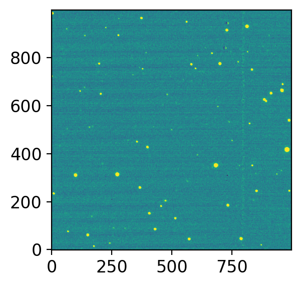
This itself is of course inferior to ds9 and ginga, because we cannot do much interactive works.
Tip
If you want to use interactive Jupyter, do %matplotlib notebook or %matplotlib widget for Jypyter notebook and Jupyter-lab, respectively. Search for the Internet for details.
1.3. Making New FITS and Saving#
Consider, for some reason, you cropped the data and take a square-root, and want to save this as a FITS file. There are few ways to do this:
The most primitive way is to use python indexing to select some region, convert it to
astropy.fits.PrimaryHDUobject and save it.A better way is to use some pre-made functions.
Such as
astropy.nddata.CutOut2D. Unfortunately, however, they do not automatically update header.
1.3.1. Using Numpy Slicing#
hdul = fits.open(allfits[0])
data = hdul[0].data
newdata = np.sqrt(data[300:400, 650:750])
print(newdata.shape)

fig, axs = plt.subplots(1, 2, figsize=(5, 3), sharex=False, sharey=False, gridspec_kw=None)
vis.norm_imshow(axs[0], newdata, zscale=True)
vis.norm_imshow(axs[1], newdata, zscale=False, stretch='sqrt')

plt.tight_layout()
(100, 100)
/var/folders/b1/mdnx6bfn6_v7p70xc3hpc9vh0000gn/T/ipykernel_13164/2916193753.py:3: RuntimeWarning: invalid value encountered in sqrt
  newdata = np.sqrt(data[300:400, 650:750])
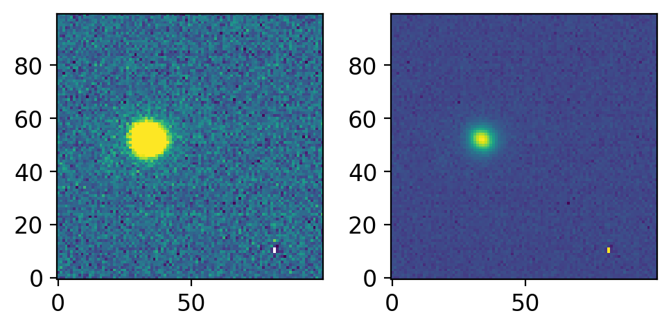
Note that [300:400, 650:750] will select 100x100 pixels.
Once you are happy, you can save it by the following code:
newhdu = fits.PrimaryHDU(data=newdata, header=hdul[0].header)
newhdu.writeto(Path("tmp") / "test.fits", overwrite=True, output_verify='fix')
For the options when writing with .writeto, refer to the official document).
Notes on Python numpy axis
Python array has the axis orientation shown below.
Example:
(x, y) = (2, 3)indata(the pixel at 2nd column 3rd row) must be accessed bydata[2, 1](xy swapped, decrease by 1)Python slice contains the beginning index, but excludes the last index (
data[:3, 0]will result in[data[0, 0], data[1, 0], data[2, 0]], but NOTdata[3, 0]). Therefore,(x, y) = (2~3, 4~7)(the 2 x 4 pixels at 2nd-3rd columns & 4th-7th rows) must be accessed bydata[3:7, 1:3].TIP: So you may reach a general formula. To select
(x, y) = (x1~x2, y1~y2), you have to usedata[y1-1:y2, x1-1:x2].
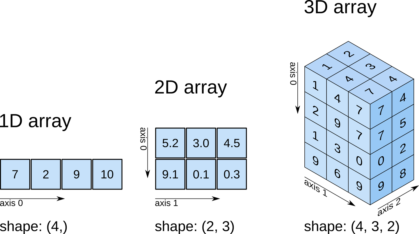 ▲ Note the axes order and indexing for 2-D array
1.3.2. Using astropy.nddata.Cutout2D#
Tutorials on this module can be found at the official documentation on image utilities. Also the official doc.
class astropy.nddata.Cutout2D(
    data, position, size, wcs=None, mode='trim', fill_value=nan, copy=False
)
Cutout2D is not easy to deal with — it is not a CCDData nor HDU-like type. Thus, I made a simple function to convert it to CCDData.
from astropy.nddata import Cutout2D
from astropy.wcs import WCS


def cut_ccd(ccd, position, size, mode="trim", fill_value=np.nan, warnings=True):
    """ Converts the Cutout2D object to proper CCDData."""
    cutout = Cutout2D(
        data=ccd.data, position=position, size=size,
        wcs=getattr(ccd, "wcs", WCS(ccd.header)),
        mode=mode, fill_value=fill_value, copy=True,
    )
    # Copy True just to avoid any contamination to the original ccd.

    nccd = CCDData(data=cutout.data, header=ccd.header.copy(),
                   wcs=cutout.wcs, unit=ccd.unit)
    ny, nx = nccd.data.shape
    nccd.header["NAXIS1"] = nx
    nccd.header["NAXIS2"] = ny
    nccd.header["LTV1"] = nccd.header.get("LTV1", 0) - cutout.origin_original[0]
    nccd.header["LTV2"] = nccd.header.get("LTV2", 0) - cutout.origin_original[1]

    return nccd


ccd = CCDData.read(allfits[0], unit="adu")
cut = cut_ccd(ccd, position=(700, 350), size=(100, 100))
print(cut.shape)
cut.data = np.sqrt(cut.data)

fig, axs = plt.subplots(1, 2, figsize=(5, 3), sharex=False, sharey=False, gridspec_kw=None)
vis.norm_imshow(axs[0], cut.data, zscale=True)
vis.norm_imshow(axs[1], cut.data, zscale=False, stretch='sqrt')
plt.tight_layout()
WARNING: FITSFixedWarning: RADECSYS= 'ICRS ' / Telescope Coordinate System
the RADECSYS keyword is deprecated, use RADESYSa. [astropy.wcs.wcs]
/var/folders/b1/mdnx6bfn6_v7p70xc3hpc9vh0000gn/T/ipykernel_13164/2203502910.py:28: RuntimeWarning: invalid value encountered in sqrt
  cut.data = np.sqrt(cut.data)
INFO: using the unit adu passed to the FITS reader instead of the unit adu in the FITS file. [astropy.nddata.ccddata]
(100, 100)
Because cut is now CCDData, you may use .write method:
cut.write(Path("tmp") / "test.fits", overwrite=True, output_verify='fix')
1.3.3. IRAF-like Slicing#
In IRAF, there is a task named IMCOPY.
I made two similar functions:
ysfitsutilpy.imslice(ccd, trimsec, fill_value=None, order_xyz=True,
                     update_header=True, verbose=False)
and
ysfitsutilpy.imcopy(inputs, trimsecs=None, outputs=None, extension=None,
                    return_ccd=True, dtype=None, update_header=True, **kwargs)
imslice is the most basic, pythonic way of slicing a part of %he image based on trimsec. trimsec can be one of
str: The FITS convention section to trim (e.g., IRAF TRIMSEC).[list of] int: The number of pixels to trim from the edge of the image (bezel). If list, it must be [bezel_lower, bezel_upper].[list of] slice: The slice of each axis (slice(start, stop, step))
imcopy is basically a copycat of IRAF, and it uses imslice under the hood, so you may just stick to imslice unless you have specific reasons. It accepts the [list of] file name[s] or CCDData.
ccd = CCDData.read(allfits[0], unit="adu")
cut = yfu.imslice(ccd, trimsec="[650:749, 300:399]")
print(cut.shape)
cut.data = np.sqrt(cut.data)

fig, axs = plt.subplots(1, 2, figsize=(5, 3), sharex=False, sharey=False, gridspec_kw=None)
vis.norm_imshow(axs[0], cut.data, zscale=True)
vis.norm_imshow(axs[1], cut.data, zscale=False, stretch='sqrt')
plt.tight_layout()
INFO: using the unit adu passed to the FITS reader instead of the unit adu in the FITS file. [astropy.nddata.ccddata]
(100, 100)
WARNING: FITSFixedWarning: RADECSYS= 'ICRS ' / Telescope Coordinate System
the RADECSYS keyword is deprecated, use RADESYSa. [astropy.wcs.wcs]
/var/folders/b1/mdnx6bfn6_v7p70xc3hpc9vh0000gn/T/ipykernel_13164/684114016.py:4: RuntimeWarning: invalid value encountered in sqrt
  cut.data = np.sqrt(cut.data)
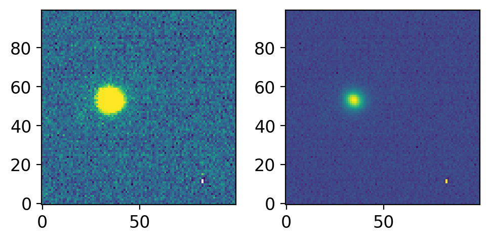
Note than you had to use 749 and 399 instead of 750 and 400. This is because the traditional FITS section (IRAF section) is 1-indexing, and includes the last number. For example, to select the first pixel, python would use [0:1, 0:1] while traditional IRAF would use [1:1, 1:1].
There is a tool to convert IRAF-like section into python, but not the inverse.
import astro_ndslice as nds
arr2d = np.arange(100).reshape(10,10)
a_slice = nds.slice_from_string('[1:3, 1:4]', fits_convention=True)
arr2d[a_slice]
array([[ 0,  1,  2],
       [10, 11, 12],
       [20, 21, 22],
       [30, 31, 32]])
a_slice = nds.slice_from_string('[1:10:2, 1:4]', fits_convention=True)
arr2d[a_slice]
array([[ 0,  2,  4,  6,  8],
       [10, 12, 14, 16, 18],
       [20, 22, 24, 26, 28],
       [30, 32, 34, 36, 38]])