2. 2-D Backgrounds

2.1. SExtractor

So far, you have learned how to estimate the background (or so-called the “sky” value) at a single star, using the annulus. Although this works sufficiently good for most of the use cases, sometimes you need 2-D fitting to the background pixels, and make a 2-D background. An example will be the target in a nebulous background or galaxy.

2.1.1. Introduction

The most widely used algorithm uses SExtractor first developed by Bertin & Arnouts (1996). The name came from “source extractor”, and thus this software’s primary goal is to extract sources (including stars, galaxies, asteroids, etc).

There are two important parts of SExtractor:

1. Estimation of the spatially varying background and

2. Automatic recognition of the sources (i.e., properties including shape, flux, etc).

A general implementation of background estimation in photutils (photutils.background) includes SExtractor-like background estimation (this will be covered in this note). The second part, source recognition (in photutils, it is implemented to photutils.segmentation) is covered in Extended Sources lecture note.

2.1.2. Documentations

There are two bibles for SExtractor and I link those for you just in case you need to use it for historical reasons:

1. Official online manual // official PDF manual from astromatic.net

   • Note that the readthedocs web can be converted to PDF (here).

2. a note called “Source Extractor for Dummies”.

You may also find them from our references.

2.1.3. Implementations in Python

In python, there are two widely used versions to mimic SExtractor:

1. photutils

2. sep (Source Extractor in Python) (the paper on JOSS)

The pros and cons of these are clear: photutils gives you more freedom, but is much slower then sep. sep uses numpy only and is much faster (see benchmark). However, sep can only do very basic calculations. I personally use sep for most works because it’s faster.

Benchmark on my mac

sep is about 70+ times faster on my mac:

$ python bench.py
test image shape: (1024, 1024)
test image dtype: float32
measure background:  12.34 ms
subtract background:   3.38 ms
background array:   6.94 ms
rms array:   5.21 ms
extract:  88.87 ms  [1167 objects]

sep version:       1.10.0
photutils version: 0.7.1

| test                    | sep             | photutils       | ratio  |
|-------------------------|-----------------|-----------------|--------|
| 1024^2 image background |        11.68 ms |       851.76 ms |  72.94 |
| circles  r= 5  subpix=5 |    3.40 us/aper |   45.30 us/aper |  13.31 |
| circles  r= 5  exact    |    3.89 us/aper |   45.76 us/aper |  11.76 |
| ellipses r= 5  subpix=5 |    3.89 us/aper |   75.29 us/aper |  19.37 |
| ellipses r= 5  exact    |   10.88 us/aper |   63.71 us/aper |   5.85 |

2.2. SExtractor Algorithm

Basic algorithm is explained in this section of the photutils documentation (as well as the SExtractor documentations linked above). SExtractor background estimation is done like this:

1. Chop image into a low-resolution image

   • In case of the axis length is not an integer multiple of corresponding box_size, you have to specify the option (edge_method). But it is highly recommended not to make such situation, so set box_size carefully.

2. For each box (“pad”) having box_size, do a median filtering with given filter size.

   • The median filter will use numpy.nan for “outside-pad” pixels. FYI, the photutils.Background2D source code uses scipy.ndimage.generic_filter, and has the following code:

   self.background_mesh = generic_filter(
           self.background_mesh, nanmedian_func, size=self.filter_size,
           mode='constant', cval=np.nan)
   

3. Do the sigma-clipping based on sigma_clip to each of the pixel within the box after this median filtering.

   • The clipping is done from median, not from mean.

4. For the low-resolution image, do an interpolation to make a background map (size identical to the original image)

   • By default, 3rd order spline fitting is used (as SExtractor default). In photutils, it is called BkgZoomInterpolator

   • Unlike median filtering, it has cval=0.0, so the values outside the range of interpolation is considered as zero-valued pads.

   • To change this, use the parameter interpolator.

5. You may need some uncertainty map for the background estimation uncertainty, which is done by tuning the paramter bkgrms_estimator. It has the input StdBackgroundRMS by default. This just calculates the sample standard deviation of the sigma-clipped data within each pad, and takes it as the pad’s background estimation RMS (roughly equal to what we call “uncertainty”). Then this low-resolution error map is also interpolated by the same way as the background value map.

Here, the low-resolutioned image (and sometimes the “tile” or pixel of this low-res image) is called background mesh, pad, or box.

2.2.1. A Detailed Explanation

For example, say the image was 1000 by 1000 pixel, and you set box_size=(50, 25). Then a low-resolution image consists of 20 by 40 “pads” or “meshes” will be made. Each pad will of course have size of 50 by 25.

If filter_size=3 (eqauivalent to use filter_size=(3, 3)), a 3 by 3 median filter will be used to reduce sharp noised pixels at each pad. After the median filtering of a pad, the image size is still 50 by 25.

Within each of this median-filtered pad, a sigma-clipping is performed. If too many pixels inside a pad is rejected, that pad is rejected for background estimation. By default, photutils.Background2D takes exclude_mesh_percentile=10, which means the pad with more than 10% of pixels are rejected will be rejected.

Then the representative background value from each pad (which has already been median filtered and sigma-clipped) by the following algorithm:

1. Use 2.5*median - 1.5*mean of each pad.

2. If (mean-median)/std > 0.3, use median.

This is done by SExtractorBackground in photutils. Of course there are other options. Check the list of API. N.B.: SExtractor user manual has a typo at page 17, photutils mentions (link).

Once the sky value is set for each pad, it does spline fitting of order 3 to the low-resolution map, i.e., the 20 by 40 image. Then by this fitting, the sky value is given to each of the pixel, i.e., the “sky map” of 1000 by 1000 pixel.

For the sky value at each pixel, we should have some uncertainty. As a rule-of-thumb, the standard deviation of the median filtered and sigma-clipped image is used. For each pad, this value is saved as a representative error, so we have 20x40 error map. The 3rd order spline fitting is also done for this error map. Then we finally have the “sky error map” of 1000x1000 pixel.

Note

If you are familiar with the photutils code, you may wonder what will happen if you put sigma_clip to the Background2D and the SExtractorBackground. The bkg_estimator part of this Background2D document says the sigma clipping parameter from SExtractorBackground will be ignored.

Important

Before proceed, please do the followings:

1. Read and follow the documentation and tutorial at photutils/background estimation.

2. Read and follow the documentation and tutorial at sep/Background subtraction (only until Background subtraction will be enough).

%load_ext version_information
import time
now = time.strftime("%Y-%m-%d %H:%M:%S (%Z = GMT%z)")
print(f"This notebook was generated at {now} ")

vv = %version_information astropy, numpy, scipy, matplotlib, astroquery, photutils, version_information
for i, pkg in enumerate(vv.packages):
    print(f"{i} {pkg[0]:10s} {pkg[1]:s}")

This notebook was generated at 2023-05-09 15:37:03 (KST = GMT+0900) 

0 Python     3.10.10 64bit [Clang 14.0.6 ]
1 IPython    8.13.2
2 OS         macOS 13.1 arm64 arm 64bit
3 astropy    5.2.2
4 numpy      1.24.3
5 scipy      1.10.1
6 matplotlib 3.7.1
7 astroquery 0.4.7.dev8597
8 photutils  1.6.0
9 version_information 1.0.4

from IPython.core.interactiveshell import InteractiveShell
from IPython import get_ipython
%config InlineBackend.figure_format = 'retina'
InteractiveShell.ast_node_interactivity = 'last_expr'
ipython = get_ipython()
from pathlib import Path

import numpy as np

from matplotlib import pyplot as plt
from matplotlib import rcParams

plt.style.use('default')
plt.rcParams.update({
    'font.family': 'latin modern math', 'font.size':12, 'mathtext.fontset':'stix', 
    'axes.formatter.use_mathtext': True, 'axes.formatter.limits': (-4, 4),
    'axes.grid': True, 'grid.color': 'gray', 'grid.linewidth': 0.5, 
    'xtick.top': True, 'ytick.right': True, 
    'xtick.direction': 'inout', 'ytick.direction': 'inout',
    'xtick.minor.size': 2.0, 'ytick.minor.size': 2.0,  # default 2.0
    'xtick.major.size': 4.0, 'ytick.major.size': 4.0,  # default 3.5
    'xtick.minor.visible': True, 'ytick.minor.visible': True
})

from astropy.io import fits
from astropy.stats import sigma_clipped_stats, SigmaClip

from photutils.background import Background2D

import sep
import ysfitsutilpy as yfu

import _tool_visualization as vis

FIGPATH = Path("figs")
DATAPATH = Path("../../Tutorial_Data")
fpath = DATAPATH/"SNUO_STX16803-kw4-4-4-20190602-135247-R-60.0_bdfw.fits"

box = 32
filt = 3

bkg_path = fpath.parent / (fpath.name[:-5] + '_bkg.png')
png_path = fpath.parent / (fpath.name[:-5] + '.png')
hdu = fits.open(fpath)[0]
data = hdu.data

avg, med, std = sigma_clipped_stats(data, sigma=3, maxiters=5)
thresh = med + 5 * std
mask = (data > thresh)  # mask = True when pixel has high signal (possibly a celestial object)

2.3. Sky Estimation by photutils.Background2D

Basically the sigma_clip parameter below has almost no effect, because we already have masked all high-valued pixels using mask. I put it here just for your future convenience.

bkg_sex = Background2D(
    data,
    box_size=box,
    mask=mask,
    filter_size=filt,
    exclude_percentile=5,
    # sigma_clip=SigmaClip(sigma=3, maxiters=5, cenfunc='median', stdfunc='std')
)
bkgsub_sex = data - bkg_sex.background

fig, axs = plt.subplots(2, 3, figsize=(10, 8))

data2plot = [
    dict(ax=axs[0, 0], arr=data, title="Original data"),
    dict(ax=axs[0, 1], arr=bkg_sex.background, title=f"bkg (filt={filt:d}, box={box:d})"),
    dict(ax=axs[0, 2], arr=bkgsub_sex, title="bkg subtracted"),
    dict(ax=axs[1, 0], arr=mask, title=f"Mask (pix > {thresh:.1f})"),
    dict(ax=axs[1, 1], arr=bkg_sex.background_mesh, title="bkg mesh"),
    dict(ax=axs[1, 2], arr=10*bkg_sex.background_rms, title="10 * bkg RMS")
]

for dd in data2plot:
    im = vis.zimshow(dd['ax'], dd['arr'])
    vis.colorbaring(fig, dd['ax'], im)
    dd['ax'].set_title(dd['title'])

# bkg_sex.plot_meshes(ax=axs[0, 1])

try:
    axs[1, 1].plot(*np.where(np.isnan(bkg_sex.mesh_nmasked))[::-1], 'rx', ms=5)
except AttributeError:
    print("No mesh (pad) is masked ")

plt.tight_layout()
# plt.savefig(FIGPATH / "sex_bkg_01.png", bbox_inches='tight')

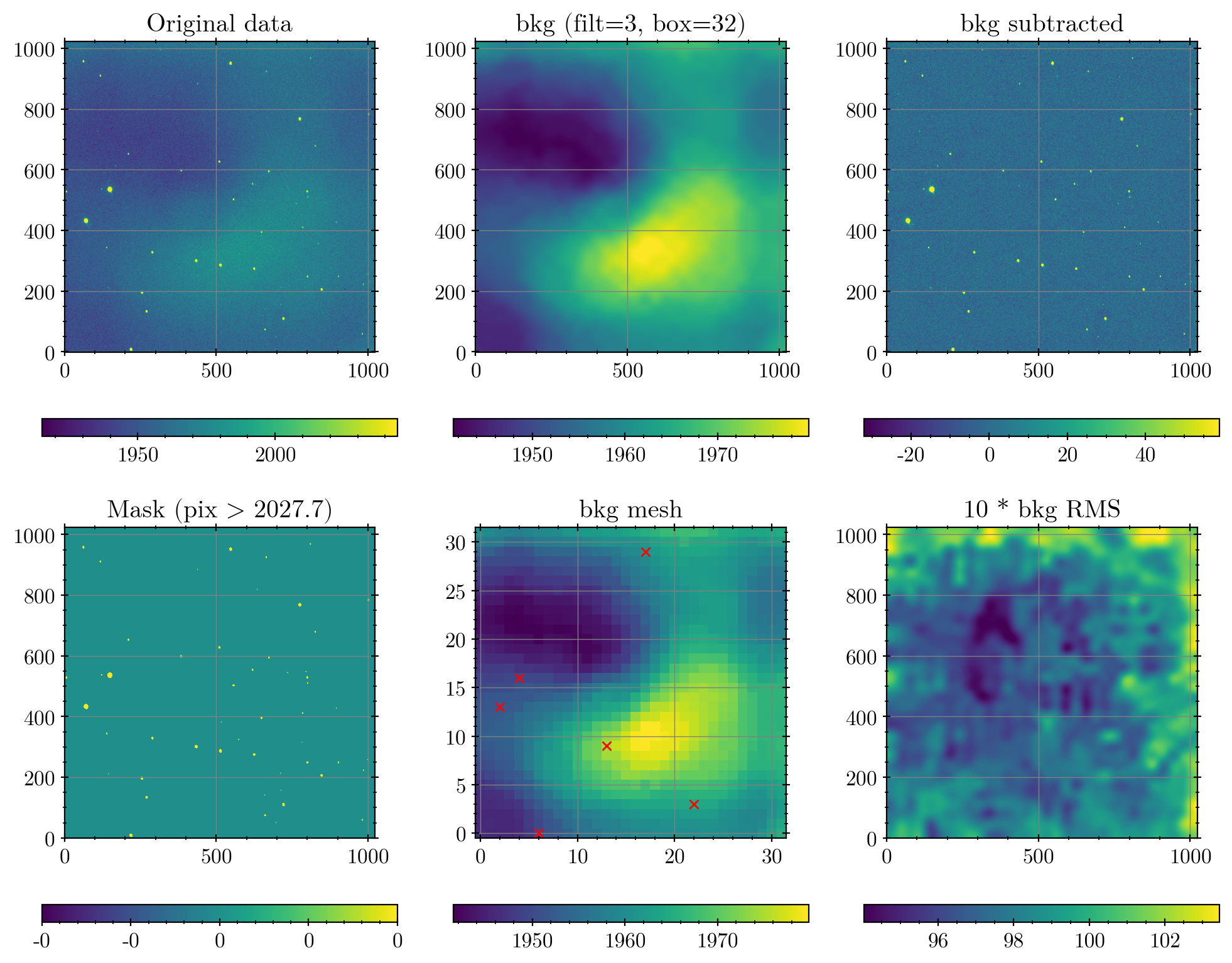
Figure:

• Top left is the original image.

• Top center is the estimated background (note the color-bar scale are different). This is the result of the BkgZoomInterpolator for the bottom center image.

• Top right is the image after the background subtraction.

• Bottom left shows the masked pixels by the 5-sigma threshold (see code). These masked (yellow) pixels are not used for sigma-clippin in the corresponding mesh (pad).

• Bottom center shows the low-resolution background mesh. Red cross shows the mesh that are not used for background estimation because too many pixels are removed from masking or sigma-clipping (including objects or highly noisy meshes).

• Bottom right shows the RMS (sqrt(sum(mesh's median - pixel value)) within mesh, and interpolate them) multiplied by 10. Note the RMS is generally low when sky values are low (Poisson noise).

In the code above, I used exclude_percentile=5 (which affects the red-crosses in the bottom center image). That is, if more than 5% of the pixels in the mesh (32 x 32 pixels, so 5% of it means 51.2) are masked or sigma-clipped, that mesh is not used in the background estimation interpolation.

Practice

What happens if exclude_percentile=10?

2.4. Sky Estimation from sep

There are some caveats which may help you when you start doing research using sep: sep is picky when it comes to the input data types. Read the note in the sep documentation. I recommend you to use a short code snippet such as

# data = # The data you want to use (e.g., ccd.data)
data = None if data is None else np.ascontiguousarray(data)
# OR
data = data.byteswap(inplace=True).newbyteorder()

(excerpt from ysphotutilpy). Below we have the non-native byte order error, so I used ``.byteswap().newbyteorder()`.

bkg_sep = sep.Background(
    data.byteswap().newbyteorder(),
    mask=mask, bw=box, bh=box, fw=filt, fh=filt
)

bkgsub_sep = data - bkg_sep.back()

fig, axs = plt.subplots(2, 3, figsize=(10, 8))
axs[1, 1].axis("off")

data2plot = [
    dict(ax=axs[0, 0], arr=data, title="Original data"),
    dict(ax=axs[0, 1], arr=bkg_sep.back(), title=f"bkg (filt={filt:d}, box={box:d})"),
    dict(ax=axs[0, 2], arr=bkgsub_sep, title="bkg subtracted"),
    dict(ax=axs[1, 0], arr=mask, title=f"Mask (pix > {thresh:.1f})"),
    dict(ax=axs[1, 2], arr=10*bkg_sep.rms(), title="10 * bkg RMS")
]

for dd in data2plot:
    im = vis.zimshow(dd['ax'], dd['arr'])
    vis.colorbaring(fig, dd['ax'], im)
    dd['ax'].set_title(dd['title'])

plt.tight_layout()
# plt.savefig(FIGPATH / "sex_bkg_01.png", bbox_inches='tight')

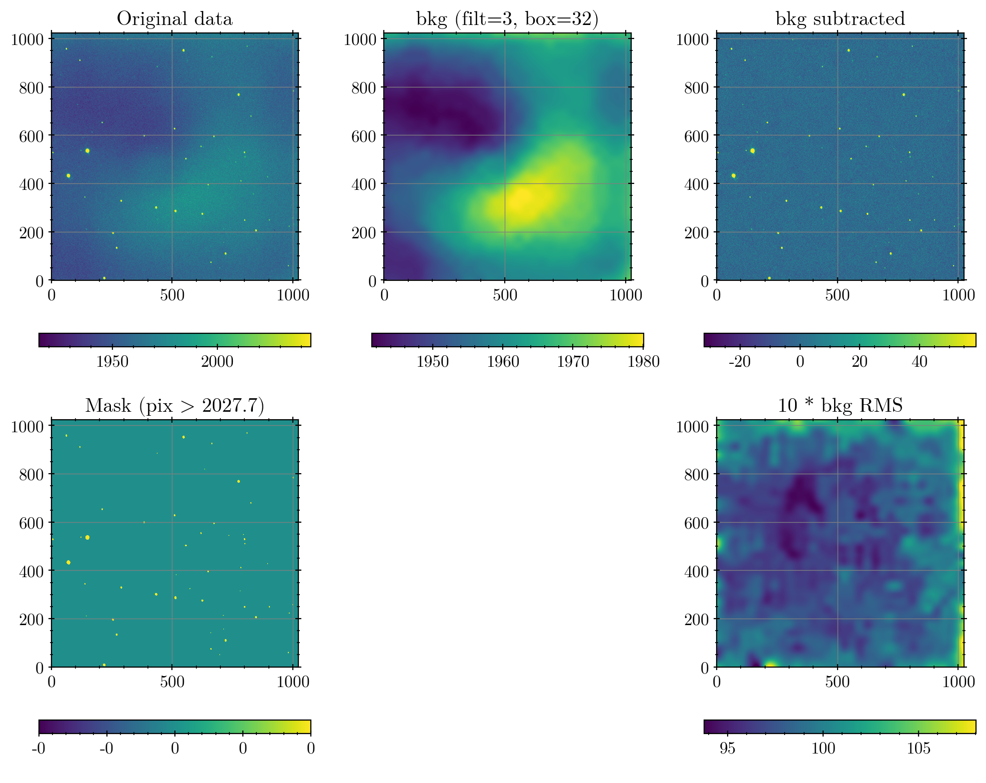
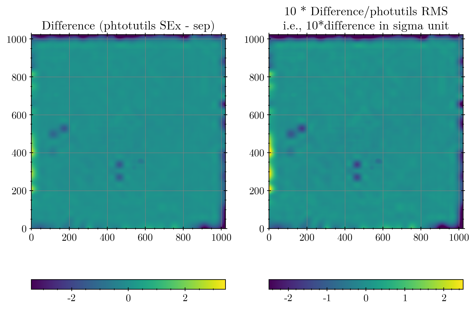
Note the bottom center plot is not plotted, because the mesh information is not provided in sep. The difference in background values from the two methods:

diff = bkg_sex.background - bkg_sep.back()
ss = yfu.give_stats(diff)
print("Statistics of the difference")
for k, v in ss.items():
    print(f"{k:>14s}: {v}")

fig, axs = plt.subplots(1, 2, figsize=(8, 6))

absmax = np.max(np.abs(diff))
im0 = axs[0].imshow(diff, origin='lower', vmin=-absmax/2, vmax=absmax/2)
vis.colorbaring(fig, axs[0], im0)

im1 = axs[1].imshow(10*diff/bkg_sex.background_rms, origin='lower', vmin=-2.5, vmax=2.5)
vis.colorbaring(fig, axs[1], im1)

axs[0].set(title="Difference (phtotutils SEx - sep)")
axs[1].set(title="10 * Difference/photutils RMS\ni.e., 10*difference in sigma unit")

plt.tight_layout()
plt.show()

# plt.savefig(figoutpath, dpi=300, bbox_inches = "tight")

Statistics of the difference
           num: 1048576
           min: -6.857295142906423
           max: 3.0729636590508562
           avg: -0.09737848032452191
           med: 0.0026730014051281614
           std: 0.5489521792690334
        madstd: 0.07000631371216799
   percentiles: [1, 99]
           pct: [-2.93927157  0.69085835]
        slices: None
          zmin: -0.47009813126558825
          zmax: 0.4798942741889543

Note

Why are they different? It is because sep does not have functionality as exclude_percentile. Therefore, as you can see, the sky value estimated from this mesh is slightly higher in sep so the difference map is negative. If you increase box size and/or filter size, this problem will be “smoothed out”.

Hence, the lesson you learn is, the input parameters for SExtractor-like algorithms should be carefully chosen not to ruin your final result.

Example

The difference is only about 2-3 ADU out of the sky value around 2000, i.e., only about 0.1%. The right panel of the last figure means it’s about 0.2-σ offset (NOT 2-σ) by the sky RMS. Is this a serious problem?

The answer depends. If your image has FWHM of 10 (significantly oversampled, which is sometimes the case), the aperture radius you will use can be something like 30 pixels. The circular aperture area then will be \(\pi (30)^2 \approx 3000 \,\mathrm{pix}^2\). With 1 ADU error in background, the source sum will be affected by 3000 ADU! If your object is quite faint so that its true count is only, say, \(10^5\) ADU, you will have 3% systematic offset in your flux. It is not a random error, so this may cause a big trouble in your research especially if you are not aware of it.

Practice

What happens if box and/or filt are increased to, e.g., 64 and 5? What happens if decreased? Try many combinations of these.