4.4. Numpy Tutorial

4.4.1. Numpy Array

Numpy array has its own “axis” system.

import numpy as np
from matplotlib import pyplot as plt
plt.style.use('default')

Arrays

Here are some useful attributes related to arrays in Python:

• .dtype: The data type

• .shape: The shape of the array in a tuple (order is (axis0, axis1, ...))

• .ndim: The dimensionality of the array (equal to len(arr.shape))

• .size: The total size of the array (\(\prod_{i=0}^{\mathtt{array.ndim - 1}} \mathtt{array.shape[i]}\))

arr1 = np.array([1, 2, 3.])
print(f"{arr1       = }")
print(f"{type(arr1) = }")
print(f"{arr1.dtype = }")

arr1       = array([1., 2., 3.])
type(arr1) = <class 'numpy.ndarray'>
arr1.dtype = dtype('float64')

print(f"{arr1.shape = }")
print(f"{arr1.size  = }")
print(f"{arr1.ndim  = }")

arr1.shape = (3,)
arr1.size  = 3
arr1.ndim  = 1

arr2 = np.array([[1, 2, 3], [4, 5, 6]])
print(f"{arr2       = }")
print(f"{type(arr2) = }")
print(f"{arr2.dtype = }")

arr2       = array([[1, 2, 3],
       [4, 5, 6]])
type(arr2) = <class 'numpy.ndarray'>
arr2.dtype = dtype('int64')

print(f"{arr2.shape = }")
print(f"{arr2.size  = }")
print(f"{arr2.ndim  = }")

arr2.shape = (2, 3)
arr2.size  = 6
arr2.ndim  = 2

Array Generation

arange

• arange: np.arange([start, ]stop, [step, ]dtype=None)

print(np.arange(10))

[0 1 2 3 4 5 6 7 8 9]

# Use the `float` input argument to make the output array as `float`:
print(np.arange(10.)) 

[0. 1. 2. 3. 4. 5. 6. 7. 8. 9.]

print(np.arange(10, 100, 5))

[10 15 20 25 30 35 40 45 50 55 60 65 70 75 80 85 90 95]

print(np.arange(10, 100, 25, dtype='float'))

[10. 35. 60. 85.]

print(np.arange(10, 100, 25, dtype=np.float128))

---------------------------------------------------------------------------
AttributeError                            Traceback (most recent call last)
Cell In[10], line 1
----> 1 print(np.arange(10, 100, 25, dtype=np.float128))

File ~/mambaforge/envs/snuao/lib/python3.10/site-packages/numpy/__init__.py:320, in __getattr__(attr)
    317     from .testing import Tester
    318     return Tester
--> 320 raise AttributeError("module {!r} has no attribute "
    321                      "{!r}".format(__name__, attr))

AttributeError: module 'numpy' has no attribute 'float128'

print(np.arange(10, 100, 25, dtype='float32'))

[10. 35. 60. 85.]

CAVEAT for arange

A potential issue related to numerical precision arises with the arange function in certain cases. This problem is discussed in detail in this issue.

np.arange(1, 1.6, 0.1)
# You would expect it ends with 1.5, but actually 1.6 is in this array!!!
# WTF!? See the link above.

array([1. , 1.1, 1.2, 1.3, 1.4, 1.5, 1.6])

linspace

• linspace: np.linspace(start, stop, num=50, endpoint=True, retstep=False, dtype=None, axis=0)

# Frequent usage is just ``np.linspace(start, stop, num)``
np.linspace(0, 10, num=5, endpoint=True)

array([ 0. ,  2.5,  5. ,  7.5, 10. ])

logspace

• logspace: np.logspace(start, stop, num=50, endpoint=True, base=10.0, dtype=None, axis=0)

# Frequent usage is just ``np.logspace(start, stop, num)``
np.logspace(0, 1, num=5, endpoint=True)

array([ 1.        ,  1.77827941,  3.16227766,  5.62341325, 10.        ])

Identical to 10**(np.logspace(0, 2)):

np.testing.assert_allclose(np.logspace(0, 2), 10**(np.linspace(0, 2)))

More About Array Generation

Random Number

For generating random numbers, an initial “starting point” is required to establish a series of random numbers.

If another person uses the same seed value, they can reproduce the exact sequence of random numbers that you generated. This observation highlights the interesting nature of random numbers—they are random yet reproducible.

rand = np.random.RandomState(12345)

arr_norm_1d = rand.normal(loc=0, scale=1, size=5)
print(arr_norm_1d)

[-0.20470766  0.47894334 -0.51943872 -0.5557303   1.96578057]

arr_norm_2d = rand.normal(loc=0, scale=1, size=(3, 3))
print(arr_norm_2d)

[[ 1.39340583  0.09290788  0.28174615]
 [ 0.76902257  1.24643474  1.00718936]
 [-1.29622111  0.27499163  0.22891288]]

Check whether it’s really normally distributed when sampled many:

xx = np.linspace(-4, 4, 100)
plt.plot(xx, 1/np.sqrt(2*np.pi*1)*np.exp(-xx**2/2), 
         lw=4, alpha=0.5, label='True Gaussian')
for i in range(3):
    arr_norm_1d = rand.normal(size=50000)
    _ = plt.hist(arr_norm_1d, 100, histtype='step', density=True, label=f"Trial {i+1}")

plt.legend()

<matplotlib.legend.Legend at 0x1174a6110>

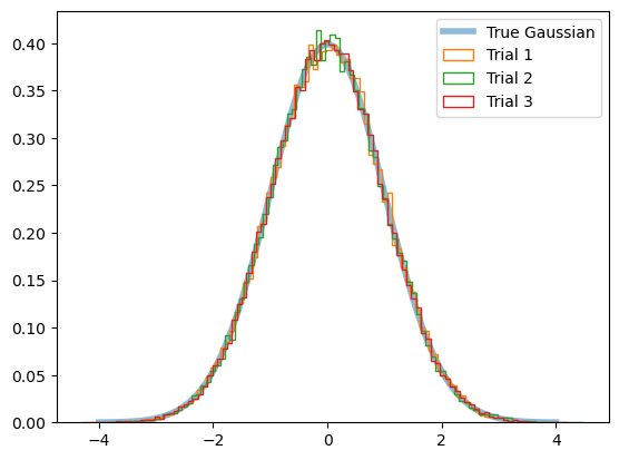
Many other distributions are also available (here).

Reshaping

arr_orig = np.arange(10)
arr_resh = arr_orig.reshape(2, 5)
print("original\n", arr_orig)
print("\nreshaped\n", arr_resh)
print("\nreshaped's shape\n", arr_resh.shape)

original
 [0 1 2 3 4 5 6 7 8 9]

reshaped
 [[0 1 2 3 4]
 [5 6 7 8 9]]

reshaped's shape
 (2, 5)

One, Zero, Empty, and Identity

reference = np.arange(9).reshape(3, 3)
ones = np.ones((3, 3))
zeros = np.zeros((3, 3))
emptys = np.empty((3, 3))
identity = np.eye(3)

print("Ones\n", ones)
print("\nZeros\n", zeros)
print("\nEmpty\n", emptys)
print("\nIdentity\n", identity)

Ones
 [[1. 1. 1.]
 [1. 1. 1.]
 [1. 1. 1.]]

Zeros
 [[0. 0. 0.]
 [0. 0. 0.]
 [0. 0. 0.]]

Empty
 [[20.  0. -0.]
 [ 0.  7. -0.]
 [ 0.  0.  1.]]

Identity
 [[1. 0. 0.]
 [0. 1. 0.]
 [0. 0. 1.]]

Using np.empty is generally not recommended due to the possibility of filling the array with “garbage” values like 1.5e-323 or 1. I personally do not know when it is necessary to use np.empty instead of np.zeros or np.ones to initialize an array.

Another useful function is xxxx_like, where xxxx can be replaced with zeros, ones, or any other desired function. This function creates a new array with the same shape and data type as the provided input array. It can be particularly helpful when you want to create a new array based on the characteristics of an existing one.

reference = np.arange(9).reshape(3, 3)
ones_like = np.ones_like(reference)
# np.ones(reference.shape)
zeros_like = np.zeros_like(reference)
emptys_like = np.empty_like((3, 3))

print("Ones_like\n", ones)
print("\nZeros_like\n", zeros)
print("\nEmpty_like\n", emptys)

Ones_like
 [[1. 1. 1.]
 [1. 1. 1.]
 [1. 1. 1.]]

Zeros_like
 [[0. 0. 0.]
 [0. 0. 0.]
 [0. 0. 0.]]

Empty_like
 [[20.  0. -0.]
 [ 0.  7. -0.]
 [ 0.  0.  1.]]

Array Indexing

Similar to usual python

a1 = np.arange(10).reshape(2, 5)
print(a1[0]) # equivalent to a1[0, :], NOT a1[:, 0]
print(a1[0, :])

[0 1 2 3 4]
[0 1 2 3 4]

print(a1[0, 1:3])
print(a1[0, ::2])  # double colon means "every other x elements"

[1 2]
[0 2 4]

print(a1[-1, :])

[5 6 7 8 9]

a1[0, 0] = -111
print(a1)

[[-111    1    2    3    4]
 [   5    6    7    8    9]]

Use [::-1] to “reverse” the array/list:

print("a1[::-1]")
print(a1[::-1])
print("\na1[:, ::-1]")
print(a1[:, ::-1])

a1[::-1]
[[   5    6    7    8    9]
 [-111    1    2    3    4]]

a1[:, ::-1]
[[   4    3    2    1 -111]
 [   9    8    7    6    5]]

# N-D to 1-D
print(a1.flatten())

[-111    1    2    3    4    5    6    7    8    9]

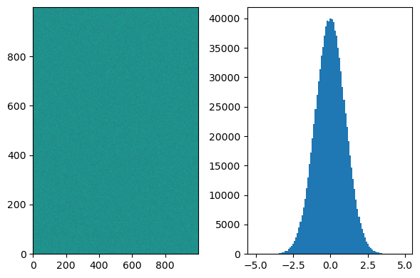
When to use flatten()?

The flatten() function in NumPy is useful when you have multi-dimensional data and you want to convert it into a one-dimensional array.

For example, consider a scenario where you have a large N-dimensional dataset, such as a 1000 x 1000 = 1,000,000 pixel image. If you want to compute a histogram of pixel values from this image, using flatten() can be beneficial.

If you don’t use flatten() in this case, it can take a considerable amount of time and may even yield unexpected results. By flattening the multi-dimensional array into a one-dimensional representation, you can efficiently compute the desired histogram without unnecessary processing or unexpected outcomes.

rand = np.random.RandomState(12345)

# Random number sampling from the standard normal distribution
data = rand.normal(size=(1000, 1000))

fig, axs = plt.subplots(1, 2, figsize=(6, 4))

axs[0].imshow(data, origin='lower', aspect='auto')
_ = axs[1].hist(data.flatten(), bins=100)

plt.tight_layout()
plt.show()

Concatenation

In general, there are not many specific use cases for directly concatenating or merging arrays using NumPy. Experienced Python users typically prefer using Python’s built-in data structures like list or tuple for intermediate concatenation and conversion to NumPy arrays at a later stage. This approach offers more flexibility and simplicity during concatenation operations. NumPy’s concatenation functions, such as np.concatenate() or np.stack(), are usually used when working specifically with NumPy arrays or during the final stages of data preparation.

a = np.arange(10)
b = np.linspace(20, 11, num=10)

print(a, b)

[0 1 2 3 4 5 6 7 8 9] [20. 19. 18. 17. 16. 15. 14. 13. 12. 11.]

print("concatenate")
print(np.concatenate([a, b]))
print("\nhstack")
print(np.hstack([a, b]))
print("\nvstack")
print(np.vstack([a, b]))

concatenate
[ 0.  1.  2.  3.  4.  5.  6.  7.  8.  9. 20. 19. 18. 17. 16. 15. 14. 13.
 12. 11.]

hstack
[ 0.  1.  2.  3.  4.  5.  6.  7.  8.  9. 20. 19. 18. 17. 16. 15. 14. 13.
 12. 11.]

vstack
[[ 0.  1.  2.  3.  4.  5.  6.  7.  8.  9.]
 [20. 19. 18. 17. 16. 15. 14. 13. 12. 11.]]

You can use axis option for concatenate, but it may give AxisError if you do axis=1 above to mimic vstack results.

4.4.2. Array Arithmetics

ref1 = np.arange(20).reshape(5, 4)
ref2 = np.arange(-19, 1).reshape(5, 4)

print(ref1)
print(ref2)

[[ 0  1  2  3]
 [ 4  5  6  7]
 [ 8  9 10 11]
 [12 13 14 15]
 [16 17 18 19]]
[[-19 -18 -17 -16]
 [-15 -14 -13 -12]
 [-11 -10  -9  -8]
 [ -7  -6  -5  -4]
 [ -3  -2  -1   0]]

Basic Arithmetics

print(2*ref1)
print(ref1**2)

[[ 0  2  4  6]
 [ 8 10 12 14]
 [16 18 20 22]
 [24 26 28 30]
 [32 34 36 38]]
[[  0   1   4   9]
 [ 16  25  36  49]
 [ 64  81 100 121]
 [144 169 196 225]
 [256 289 324 361]]

print(ref1 + ref2)

[[-19 -17 -15 -13]
 [-11  -9  -7  -5]
 [ -3  -1   1   3]
 [  5   7   9  11]
 [ 13  15  17  19]]

print(ref1 * ref2)

[[  0 -18 -34 -48]
 [-60 -70 -78 -84]
 [-88 -90 -90 -88]
 [-84 -78 -70 -60]
 [-48 -34 -18   0]]

print(ref1/ref2)

[[ -0.          -0.05555556  -0.11764706  -0.1875    ]
 [ -0.26666667  -0.35714286  -0.46153846  -0.58333333]
 [ -0.72727273  -0.9         -1.11111111  -1.375     ]
 [ -1.71428571  -2.16666667  -2.8         -3.75      ]
 [ -5.33333333  -8.5        -18.                  inf]]

/var/folders/b1/mdnx6bfn6_v7p70xc3hpc9vh0000gn/T/ipykernel_12883/2058048057.py:1: RuntimeWarning: divide by zero encountered in divide
  print(ref1/ref2)

Matrix multiplication by @

print(ref1@ref2.T)  # .T to Transpose

[[ -100   -76   -52   -28    -4]
 [ -380  -292  -204  -116   -28]
 [ -660  -508  -356  -204   -52]
 [ -940  -724  -508  -292   -76]
 [-1220  -940  -660  -380  -100]]

• NOTE: See what happens if you don’t do .T to ref2.

NaN and inf

NaN (Not a Number) and inf (infinity) are essential concepts in NumPy-related packages and have practical applications. In regular Python, performing an operation like 1 / 0 would result in an error and disrupt the program’s execution. However, in NumPy, a RuntimeWarning is raised instead, and the result is assigned as nan (not a number). This behavior allows the rest of the calculations to proceed correctly, except when encountering invalid operations.

This approach is advantageous because it enables your code to run as expected without encountering errors, eliminating the need to handle exceptions explicitly. Later, during the final stages of computation, you can easily identify and remove any results containing nan values. This allows for cleaner and more efficient code execution, as you can focus on processing valid results while discarding invalid or incomplete calculations.

ref1_ref2 = ref1/ref2
# RuntimeWarning will appear

/var/folders/b1/mdnx6bfn6_v7p70xc3hpc9vh0000gn/T/ipykernel_12883/4165815205.py:1: RuntimeWarning: divide by zero encountered in divide
  ref1_ref2 = ref1/ref2

np.isinf(ref1_ref2)

array([[False, False, False, False],
       [False, False, False, False],
       [False, False, False, False],
       [False, False, False, False],
       [False, False, False,  True]])

np.isnan(np.log(-1))

/var/folders/b1/mdnx6bfn6_v7p70xc3hpc9vh0000gn/T/ipykernel_12883/916304143.py:1: RuntimeWarning: invalid value encountered in log
  np.isnan(np.log(-1))

True

isinf = (ref1_ref2 == np.inf)  # same as np.isinf(~~)
isnan = (ref1_ref2 == np.nan)  # same as np.isnan(~~)
print(isinf)
print(isnan)

[[False False False False]
 [False False False False]
 [False False False False]
 [False False False False]
 [False False False  True]]
[[False False False False]
 [False False False False]
 [False False False False]
 [False False False False]
 [False False False False]]

To quickly chech how many nan or inf happened:

print(np.count_nonzero(np.isinf(ref1_ref2)))

1

Axis Operation

If you use numpy without utilizing axis, you are doing something wrong.

print("Original\n", ref1)
print("\nSum all\n", ref1.sum())
print("\nSum axis0\n", ref1.sum(axis=0))
print("\nSum axis1\n", ref1.sum(axis=1))

Original
 [[ 0  1  2  3]
 [ 4  5  6  7]
 [ 8  9 10 11]
 [12 13 14 15]
 [16 17 18 19]]

Sum all
 190

Sum axis0
 [40 45 50 55]

Sum axis1
 [ 6 22 38 54 70]

Many more: .min(), .max(), .mean()…

Better way is to use np.min(), etc:

print("Mean axis1", np.mean(ref1, axis=1))
print("Median axis1", np.median(ref1, axis=1))
print("Sample std axis1", np.std(ref1, axis=1, ddof=1))

Mean axis1 [ 1.5  5.5  9.5 13.5 17.5]
Median axis1 [ 1.5  5.5  9.5 13.5 17.5]
Sample std axis1 [1.29099445 1.29099445 1.29099445 1.29099445 1.29099445]

4.4.3. Masking

Basic Masking

rand = np.random.RandomState(123)
a = rand.normal(size=(5, 4))
b = rand.normal(size=(5, 4))
print(a)

[[-1.0856306   0.99734545  0.2829785  -1.50629471]
 [-0.57860025  1.65143654 -2.42667924 -0.42891263]
 [ 1.26593626 -0.8667404  -0.67888615 -0.09470897]
 [ 1.49138963 -0.638902   -0.44398196 -0.43435128]
 [ 2.20593008  2.18678609  1.0040539   0.3861864 ]]

NOTE: You should not erase any of the parentheses below:

m_a = ((-1 < a) & (a < 1))
# For "or", you can use ``|`` (called "pipe". Hit "shift + \")
in1sig = np.count_nonzero(m_a)
in1sig_ratio = in1sig / a.size

print("Mask\n", m_a)
print("\nMasked values\n", a[m_a])
print("\nIn 1-sigma ratio\n", in1sig_ratio)

Mask
 [[False  True  True False]
 [ True False False  True]
 [False  True  True  True]
 [False  True  True  True]
 [False False False  True]]

Masked values
 [ 0.99734545  0.2829785  -0.57860025 -0.42891263 -0.8667404  -0.67888615
 -0.09470897 -0.638902   -0.44398196 -0.43435128  0.3861864 ]

In 1-sigma ratio
 0.55

Statistically, 68.xx % should be in 1-sigma range. We have only 20 samples, so it’s a small-number statistics, and may significanlty differ from 68%.

data_quality = np.ones_like(b).astype(bool)
data_quality[2, 1:3] = False
data_quality

array([[ True,  True,  True,  True],
       [ True,  True,  True,  True],
       [ True, False, False,  True],
       [ True,  True,  True,  True],
       [ True,  True,  True,  True]])

Advanced Masking

If you just do b[data_quality], the dimension will be reduced to 1-D, which makes it difficult to operate (e.g., average) with a. Then, we replace these with nan:

b_nan = b.copy()
b_nan[~data_quality] = np.nan
b_nan

array([[ 0.73736858,  1.49073203, -0.93583387,  1.17582904],
       [-1.25388067, -0.6377515 ,  0.9071052 , -1.4286807 ],
       [-0.14006872,         nan,         nan, -2.79858911],
       [-1.7715331 , -0.69987723,  0.92746243, -0.17363568],
       [ 0.00284592,  0.68822271, -0.87953634,  0.28362732]])

np.mean([a, b_nan], axis=0)

array([[-0.17413101,  1.24403874, -0.32642769, -0.16523283],
       [-0.91624046,  0.50684252, -0.75978702, -0.92879666],
       [ 0.56293377,         nan,         nan, -1.44664904],
       [-0.14007174, -0.66938962,  0.24174024, -0.30399348],
       [ 1.104388  ,  1.4375044 ,  0.06225878,  0.33490686]])

Whole data is ignored at least one is nan. How to just ignore nan and take average of non-nan values?

np.nanmean([a, b_nan], axis=0)

array([[-0.17413101,  1.24403874, -0.32642769, -0.16523283],
       [-0.91624046,  0.50684252, -0.75978702, -0.92879666],
       [ 0.56293377, -0.8667404 , -0.67888615, -1.44664904],
       [-0.14007174, -0.66938962,  0.24174024, -0.30399348],
       [ 1.104388  ,  1.4375044 ,  0.06225878,  0.33490686]])

nanmean, nanmedian, etc are much slower:

%timeit np.mean([a, b_nan], axis=0)
%timeit np.nanmean([a, b_nan], axis=0)

5.26 µs ± 78.9 ns per loop (mean ± std. dev. of 7 runs, 100,000 loops each)

12.8 µs ± 376 ns per loop (mean ± std. dev. of 7 runs, 100,000 loops each)

NOTE: If you want to test the time spent on the whole cell, use %%timeit.

TIP: There’s a package called bottleneck which is much faster than numpy in many cases.

Masked Array

a_masked = np.ma.array(data=a, mask=m_a)
b_masked = np.ma.array(data=b, mask=~data_quality)
print(type(a_masked))

<class 'numpy.ma.core.MaskedArray'>

a_masked

masked_array(
  data=[[-1.0856306033005612, --, --, -1.5062947139180922],
        [--, 1.651436537097151, -2.426679243393074, --],
        [1.2659362587055338, --, --, --],
        [1.4913896261242878, --, --, --],
        [2.205930082725455, 2.1867860889737862, 1.004053897878877, --]],
  mask=[[False,  True,  True, False],
        [ True, False, False,  True],
        [False,  True,  True,  True],
        [False,  True,  True,  True],
        [False, False, False,  True]],
  fill_value=1e+20)

b_masked

masked_array(
  data=[[0.7373685758962422, 1.490732028150799, -0.9358338684023914,
         1.1758290447821034],
        [-1.2538806677490124, -0.6377515024534103, 0.9071051958003014,
         -1.4286807002259692],
        [-0.1400687201886661, --, --, -2.7985891054607244],
        [-1.771533104509847, -0.6998772345979173, 0.9274624317585825,
         -0.1736356827902158],
        [0.0028459158968110196, 0.688222711102285, -0.8795363430090519,
         0.283627323807291]],
  mask=[[False, False, False, False],
        [False, False, False, False],
        [False,  True,  True, False],
        [False, False, False, False],
        [False, False, False, False]],
  fill_value=1e+20)

a_masked.mask

array([[False,  True,  True, False],
       [ True, False, False,  True],
       [False,  True,  True,  True],
       [False,  True,  True,  True],
       [False, False, False,  True]])

a_masked.data

array([[-1.0856306 ,  0.99734545,  0.2829785 , -1.50629471],
       [-0.57860025,  1.65143654, -2.42667924, -0.42891263],
       [ 1.26593626, -0.8667404 , -0.67888615, -0.09470897],
       [ 1.49138963, -0.638902  , -0.44398196, -0.43435128],
       [ 2.20593008,  2.18678609,  1.0040539 ,  0.3861864 ]])

For masked array, numpy automatically ignore “maked” ones when do any arithmentics

print(np.mean(a), np.mean(a_masked))

0.11441773195529015 0.5318808812103737

When two masked arrays are operated, mask is mask1 | mask2 | ...:

a_masked + b_masked

masked_array(
  data=[[-0.348262027404319, --, --, -0.33046566913598885],
        [--, 1.013685034643741, -1.5195740475927728, --],
        [1.1258675385168677, --, --, --],
        [-0.2801434783855592, --, --, --],
        [2.208775998622266, 2.8750088000760714, 0.12451755486982519, --]],
  mask=[[False,  True,  True, False],
        [ True, False, False,  True],
        [False,  True,  True,  True],
        [False,  True,  True,  True],
        [False, False, False,  True]],
  fill_value=1e+20)

4.4.4. File I/O

Although generally it’s recommended to do file i/o (input/output, which means “saveing/loading”) using pandas or other packages, numpy also has file i/o tools.

np.save("test_a", a)

The masked array is not savable: np.save("test_a_masked", a_masked) will give you an Error.

np.load("test_a.npy")

array([[-1.0856306 ,  0.99734545,  0.2829785 , -1.50629471],
       [-0.57860025,  1.65143654, -2.42667924, -0.42891263],
       [ 1.26593626, -0.8667404 , -0.67888615, -0.09470897],
       [ 1.49138963, -0.638902  , -0.44398196, -0.43435128],
       [ 2.20593008,  2.18678609,  1.0040539 ,  0.3861864 ]])

with open("test_data.csv", "w+") as ff:
    ff.write('''
1,2.3,C
2,1.9,A
3,3.3,AB
4,3.0,A
5,1.2,AB
''')

data = np.genfromtxt("test_data.csv", 
                     delimiter=',', 
                    )
print(data)

[[1.  2.3 nan]
 [2.  1.9 nan]
 [3.  3.3 nan]
 [4.  3.  nan]
 [5.  1.2 nan]]

If str data is also required, it gets dirty:

data = np.genfromtxt("test_data.csv", 
                     delimiter=',', 
                     dtype=bytes
                    ).astype(str)
print(data)

[['1' '2.3' 'C']
 ['2' '1.9' 'A']
 ['3' '3.3' 'AB']
 ['4' '3.0' 'A']
 ['5' '1.2' 'AB']]

values = data[:, 1].astype(float)
print(values)

[2.3 1.9 3.3 3.  1.2]

Much more details are at the official doc