5. Querying from the Catalog

If WCS(World Coordinate System: converts image XY pixel to, e.g., RA/DEC. See slides 4-7 of this, for example) is properly implemented, we should be able to find stars in the image automatically.

astroquery is an astropy-affiliated python package for such query.

Here I will demonstrate how to query Pan-STARRS DR2 and Gaia catalog, which are two of the widely used catalogs as of 2023.

And in the later part, I will show how to use JPL HORIZONS, that is used for querying the ephemerides (positional information of celestial objects) of solar system objects.

%load_ext version_information
import time
now = time.strftime("%Y-%m-%d %H:%M:%S (%Z = GMT%z)")
print(f"This notebook was generated at {now} ")

vv = %version_information astropy, numpy, scipy, matplotlib, astroquery, photutils, version_information
for i, pkg in enumerate(vv.packages):
    print(f"{i} {pkg[0]:10s} {pkg[1]:s}")

This notebook was generated at 2023-05-09 15:36:36 (KST = GMT+0900) 

0 Python     3.10.10 64bit [Clang 14.0.6 ]
1 IPython    8.13.2
2 OS         macOS 13.1 arm64 arm 64bit
3 astropy    5.2.2
4 numpy      1.24.3
5 scipy      1.10.1
6 matplotlib 3.7.1
7 astroquery 0.4.7.dev8597
8 photutils  1.6.0
9 version_information 1.0.4

# %matplotlib notebook
from IPython.core.interactiveshell import InteractiveShell
from IPython import get_ipython
%config InlineBackend.figure_format = 'retina'
InteractiveShell.ast_node_interactivity = 'last_expr'
ipython = get_ipython()

from pathlib import Path

import numpy as np

from astropy import units as u
from astropy.nddata import CCDData
from astropy.coordinates import SkyCoord
from astropy.time import Time

from astroquery.gaia import Gaia
from astroquery.mast import Catalogs
from astroquery.jplhorizons import Horizons
Gaia.ROW_LIMIT = -1  # no limit

from matplotlib import pyplot as plt
from matplotlib import rcParams
plt.style.use('default')
rcParams.update({'font.size':12})

from photutils.aperture import (CircularAperture, CircularAnnulus, 
                                aperture_photometry, ApertureStats)
from photutils.detection import DAOStarFinder

import warnings
warnings.filterwarnings('ignore', category=UserWarning, append=True)

import _tool_visualization as vis

DATAPATH = Path('../../Tutorial_Data')
TMPDIR = Path('tmp')
TMPDIR.mkdir(exist_ok=True)

allfits = list(DATAPATH.glob("*p4179*.fits"))
allfits.sort()

ccd = CCDData.read(allfits[0])

WARNING: FITSFixedWarning: RADECSYS= 'ICRS ' / Telescope Coordinate System 
the RADECSYS keyword is deprecated, use RADESYSa. [astropy.wcs.wcs]

5.1. The Catalogs

Gaia (Wikipedia) is the ESA space mission that is planned to work from 2013-2025. Its main goal is to perform precise astrometry of 1 billion objects. Since it has two passbands, colorimetry has also been performed.

As of 2023, Data Realease 3 (DR3) is the most recent available data set for Gaia.

Pan-STARRS1 (also called PS1; Wikipedia) is a ground-based 1.8 m Ritchey-Chredien telescope facility at Hawaii.

As of 2023, Data Realease 2 (DR2) is the most recent available data set for PS1.

5.2. Archives

There are multiple archive services for large-scale astronomical datasets:

VizieR (Wikipedia)

A catalog service run by Université de Strasbourg/CNRS. I feel many people archive their observational results (e.g., galaxy redshift catalog, asteroid polarimetric observation results, etc) to VizieR. Sometimes, for some reasons I cannot understand, large-catalog data are not accessible from VizieR for very long time. Also, the column names in VizieR is always very different from other catalog services. You can go to here and search for gaia or ps1 for instance.

MAST (kulski Archive for Space Telescopes; Wikipedia)

A catalog survice run by STScI. I feel MAST mainly goes with space telescope data (HST, JWST, Gaia, TESS, …). Two main ground-based mission data are available, namely Pan-STARRS and VLA-FIRST.

It seems like the most official way to access Gaia is through astroquery.Gaia using TAP+ (see official website’s “PYTHON ACCESS”). Indeed, Gaia DR3 is available only from here, not from MAST.

Important

Before proceed, please read and follow the tutorials of astroquery/gaia. (only 1.1. Query object and 1.2. Cone search are enough, i.e., .query_object_async and .cone_search_async)

Also, please skim through astropy/wcs. You don’t have to know the details, but you have to know the basic usages, e.g., the basic usage shown in astropy/wcs/wcsapi.

5.3. Query Stars in the FoV

Now check if our FITS file (CCDData) has WCS information. Since in our observation, the pixel scale is roughly 0.39 arcsec per pixel. Thus, let’s query the stars within

• a circular region (so-called the cone) centered at the center of our FoV, radius of fov_radius = 0.4*diagonal_length/2. ← This is because MAST only supports cone search.

• a rectangular region centered at the center of our FoV, width and height of 0.4*width and 0.4*height, respectively. ← This is because Gaia.query_object_async supports rectangular query.

print(ccd.wcs)

pix_scale = 0.4*u.arcsec

center_xy = np.array(ccd.shape)/2
center_radec = ccd.wcs.wcs_pix2world(*center_xy, 0)
center_coo = SkyCoord(*center_radec, unit='deg')

width, height = np.array(ccd.shape)*pix_scale

print("\nCoordinate of the center of the image:\n", center_coo)

fov_radius = np.sqrt((np.array(ccd.shape)**2).sum())/2 * pix_scale

WCS Keywords

Number of WCS axes: 2
CTYPE : 'RA---TAN'  'DEC--TAN'  
CRVAL : 204.8640878996  -8.991494826739  
CRPIX : -4068.090526349  5085.76507007  
PC1_1 PC1_2  : -0.0001096993846665  -1.593373136163e-06  
PC2_1 PC2_2  : -2.91576786403e-07  0.0001095957848141  
CDELT : 1.0  1.0  
NAXIS : 999  999

Coordinate of the center of the image:
 <SkyCoord (ICRS): (ra, dec) in deg
    (204.36178211, -9.49675272)>

/Users/ysbach/mambaforge/envs/snuao/lib/python3.10/site-packages/astropy/wcs/wcs.py:3064: RuntimeWarning: cdelt will be ignored since cd is present
  description.append(s.format(*self.wcs.cdelt))

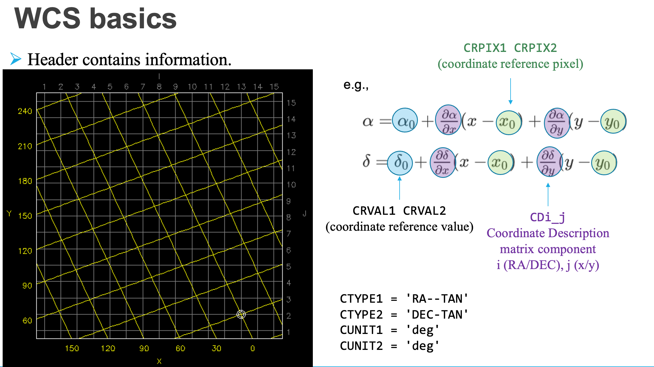
The meaning of CRVAL, CRVAL, CRPIX, and PC (you can just assume CD is identical to PC) matrices:

# =====
# If you want to use MAST, only DR2 is available as of 2023-04-26. 
# You can uncomment q_gaia line.
# Gaia DR2 needs `version=2`
# q_gaia = Catalogs.query_region(center_coo, radius=fov_radius, catalog="Gaia", version=2) 
# =====

# Set default table as DR3 and GAIA_SOURCE.
Gaia.MAIN_GAIA_TABLE = "gaiadr3.gaia_source"
q_gaia = Gaia.query_object_async(coordinate=center_coo, width=width, height=height)

# PS1 DR2 needs `data_release="dr2"`.
q_ps = Catalogs.query_region(center_coo, radius=fov_radius, catalog="Panstarrs", 
                             data_release="dr2", table="mean")
# Change some column names for convenience.
q_ps["raMean"].name = "ra"
q_ps["decMean"].name = "dec"
q_ps["gMeanPSFMag"].name = "g"
q_ps["rMeanPSFMag"].name = "r"

print("Number of results:",len(q_gaia))
print("Number of results:",len(q_ps))

INFO: Query finished. [astroquery.utils.tap.core]

Number of results: 75
Number of results: 5907

print("Number of columns in Gaia, PS1:", len(q_gaia.colnames), len(q_ps.colnames))

Number of columns in Gaia, PS1: 153 125

5.3.1. Gaia DR3

Note that Gaia DR3 GAIA_SOURCES has 153 columns! The detailed explanation of this table (GAIA_SOURCE table) in DR3 is available here. What we need are only RA, DEC, and magnitude information. For the magnitudes, the magnitude conversion methods for DR3 are given here:

\[ G - V = -0.02704 + 0.01424C - 0.2156 C^2 + 0.01426 C^3 \]

using 96413 sources (\(\sigma = 0.03017\)) and \(C := G_\mathrm{BP} - G_\mathrm{RP}\) color. The equation above is applicable to \(-0.5 < C < 5.0\).

Note

If you remember the error analysis in statistics class or theoretical part of this lecture, you may remember the uncertainty of the flux is roughly Gaussian (Poisson distribution in the limiting case). However, the magnitude is calculated by taking a logarithm to this flux. That means, the uncertainty in magnitude is not Gaussian, rigorously speaking, and the error-bars are inherently and expectedly asymmetric. Because of this, GAIA team refuses to provide any “magnitude error” value, but only provide the “flux error” value.

This is a bit annoying for most astronomers because we want to use simple error-bar for magnitudes. However, at the same time, I feel this is a declaration that astronomy is now going into a branch of precise science, not grossly approximating the asymmetric error-bar into a single number.

Warning

When you load FITS by CCDData.read, the WCS related information in the header will be deleted. Hence, you must use ccd.wcs to access the WCS information. In other words, WCS(ccd.header) will give empty WCS. This is a bit confusing, since you had to use WCS(hdu.header) in case of HDU object, as you practiced. When saving the CCDData back, WCS-related headers will be re-added.

For error analysis, note that, from Pogson’s formula:

\[ C = G_\mathrm{BP} - G_\mathrm{RP} = -2.5 \lg \frac{I_\mathrm{BP}}{I_\mathrm{RP}} \]

(I is flux). Thus, ignoring any covariance, a simple error propagation gives

\[ \Delta C \approx \frac{2.5}{\ln 10} \sqrt{ \left( \frac{dI_\mathrm{BP}}{I_\mathrm{BP}} \right)^2 + \left( \frac{dI_\mathrm{RP}}{I_\mathrm{RP}} \right)^2 } \]

and

\[ \Delta V = \sqrt{ (\Delta G)^2 + (0.01424 - 2 \times 0.2156 C + 3 \times 0.01426 C^2)^2 (\Delta C)^2 } \]

And you may also include the RMS error \(\sigma = 0.03017\) with that.

coef = np.array([-0.02704, 0.1425, -0.2156, 0.01426])
rmse = 0.03017
color = q_gaia["bp_rp"]

# Add useful columns
q_gaia["bp_snr"] = 1/q_gaia["phot_bp_mean_flux_over_error"]
q_gaia["rp_snr"] = 1/q_gaia["phot_rp_mean_flux_over_error"]
q_gaia["g_snr"] = 1/q_gaia["phot_g_mean_flux_over_error"]

# Calculate color error
q_gaia["dC"] = 2.5/np.log(10)*np.sqrt((q_gaia["rp_snr"])**2 + (q_gaia["bp_snr"])**2)

# Calculate V-mag and error
q_gaia["V"] = (
    q_gaia["phot_g_mean_mag"]
    + coef[0] + coef[1]*color + coef[2]*color**2 + coef[3]*color**3
)
q_gaia["dV"] = np.sqrt(
    2.5/np.log(10)*q_gaia["g_snr"]**2
    + (coef[1] + 2*coef[2]*color + 3*coef[3]*color**2)**2*q_gaia["dC"]**2
    + rmse**2
)

# Only select stars with good color
mask = (-0.5 < color) & (color < 5)
q1 = q_gaia["ra", "dec", "bp_rp", "g_snr", "bp_snr", "rp_snr", "dC", "V", "dV"][mask]

# Calculate x, y position
coo = SkyCoord(q1["ra"], q1["dec"], unit='deg')
q1["x"], q1["y"] = ccd.wcs.wcs_world2pix(coo.ra, coo.dec, 0)

# Remove stars outside the image
q1 = q1[(q1["x"] > 10) & (q1["x"] < ccd.shape[1]-10) 
        & (q1["y"] > 10) & (q1["y"] < ccd.shape[0]-10)]

# print
print(f"Total {len(q1)} stars")
q1.round(3)
q1

Total 65 stars

Table length=65

ra	dec	bp_rp	g_snr	bp_snr	rp_snr	dC	V	dV	x	y
deg	deg	mag
float64	float64	float32	float32	float32	float32	float32	float32	float32	float64	float64
204.352	-9.504	0.732	0.016	0.139	0.188	0.254	20.859	0.051	586.313	435.758
204.373	-9.505	2.855	0.002	0.033	0.004	0.036	16.681	0.041	399.077	428.649
204.373	-9.505	2.871	0.006	0.016	0.01	0.02	16.781	0.034	399.015	427.491
204.373	-9.505	2.748	0.005	0.245	0.087	0.282	19.131	0.205	403.101	420.853
204.35	-9.508	1.956	0.004	0.13	0.051	0.152	19.712	0.087	607.765	395.122
204.378	-9.502	0.28	0.003	0.035	0.058	0.073	19.432	0.03	355.88	450.611
204.34	-9.486	2.01	0.003	0.092	0.032	0.106	19.125	0.066	692.754	596.982
204.343	-9.514	2.116	0.005	0.116	0.037	0.132	19.665	0.082	669.384	345.025
204.341	-9.513	1.08	0.0	0.002	0.002	0.003	15.47	0.03	684.598	352.004
204.345	-9.518	1.801	0.006	0.135	0.061	0.161	20.172	0.085	650.856	304.49
204.334	-9.502	0.732	0.005	0.085	0.077	0.125	20.313	0.036	752.049	455.31
204.377	-9.523	1.174	0.002	0.013	0.009	0.017	17.866	0.031	367.571	259.337
204.35	-9.469	0.725	0.003	0.04	0.039	0.061	19.568	0.032	599.882	755.681
204.379	-9.471	1.173	0.012	0.206	0.138	0.269	20.741	0.088	338.946	728.53
204.375	-9.469	2.53	0.002	0.059	0.01	0.065	18.277	0.054	379.274	753.508
204.352	-9.467	1.924	0.001	0.019	0.008	0.023	17.426	0.032	582.302	772.492
204.376	-9.468	1.026	0.007	0.112	0.132	0.188	20.495	0.057	366.729	759.281
204.387	-9.517	0.638	0.0	0.003	0.003	0.004	15.986	0.03	273.809	314.073
204.33	-9.513	2.294	0.005	0.135	0.047	0.155	19.702	0.101	783.429	350.589
...	...	...	...	...	...	...	...	...	...	...
204.384	-9.542	1.766	0.015	0.166	0.051	0.188	20.213	0.098	306.31	90.397
204.354	-9.447	2.059	0.001	0.04	0.012	0.045	17.944	0.039	562.63	949.677
204.354	-9.547	0.941	0.001	0.011	0.008	0.015	17.691	0.03	573.426	44.983
204.313	-9.517	1.127	0.005	0.103	0.066	0.133	20.153	0.049	938.2	315.155
204.335	-9.451	1.016	0.001	0.01	0.01	0.015	17.618	0.03	730.181	914.864
204.375	-9.445	1.64	0.001	0.033	0.006	0.036	17.561	0.034	374.606	964.896
204.308	-9.506	0.996	0.0	0.001	0.001	0.002	14.891	0.03	980.531	417.518
204.31	-9.479	0.783	0.001	0.005	0.006	0.008	16.631	0.03	959.438	663.959
204.399	-9.536	0.466	0.014	0.181	0.199	0.292	20.873	0.036	167.756	139.08
204.31	-9.476	0.966	0.002	0.044	0.029	0.057	19.063	0.033	962.303	689.623
204.392	-9.45	1.706	0.003	0.076	0.039	0.093	19.268	0.053	226.356	925.276
204.386	-9.446	0.317	0.012	0.102	0.156	0.202	20.858	0.033	280.684	962.428
204.402	-9.453	0.858	0.005	0.143	0.078	0.176	20.26	0.046	139.056	892.001
204.33	-9.547	1.386	0.002	0.008	0.004	0.009	16.915	0.03	789.271	46.365
204.326	-9.449	0.959	0.001	0.004	0.004	0.006	16.488	0.03	814.182	930.355
204.391	-9.549	2.686	0.002	0.098	0.014	0.107	18.153	0.082	243.065	27.85
204.401	-9.545	0.745	0.001	0.017	0.012	0.023	17.642	0.03	150.905	61.991
204.398	-9.55	0.947	0.002	0.045	0.038	0.064	19.208	0.034	176.525	15.585
204.321	-9.549	0.664	0.004	0.064	0.068	0.102	20.012	0.033	873.151	20.835
204.41	-9.543	1.536	0.002	0.04	0.019	0.048	18.844	0.036	68.817	76.787

5.3.2. Pan-STARRS1 DR2

It seems like there are three tables available from PS1 web query API (e.g., this notebook): “mean”, “stack”, and “detection”. All the metadata can be found based on the url (see ps1metadata function), e.g., this link for the metadata of mean table.

According to Tonry+12,

\[\begin{split} V - r = 0.006 + 0.474(g-r) \quad\rightarrow\quad V = 0.006 + 0.474g + 0.526r \quad (\pm 0.012) \\ R - r = -0.138 - 0.131(g-r) \quad\rightarrow\quad R = -0.138 -0.131g + 1.131 r \quad (\pm 0.015) \end{split}\]

where g, r are the g- and r-band magnitudes in PS1 filter system, respectively. Thus,

\[\begin{split} \Delta V = \sqrt{ (0.474 \Delta g)^2 + (0.526 \Delta r)^2 } \\ \Delta R = \sqrt{ (0.131 \Delta g)^2 + (1.131 \Delta r)^2 } \end{split}\]

And you may also include the RMS error \(\sigma = 0.012\) or \(0.015\) with that.

In real science case, you must remove galaxies for differential photometry (maybe discussed later). Here, we will ignore it.

# drop stars with unknown magnitudes
q_ps = q_ps.to_pandas().dropna(subset=["g", "r"])

# Calculate V and R
q_ps["V"] = 0.006 + 0.474*q_ps["g"] + 0.526*q_ps["r"]
q_ps["R"] = -0.138 - 0.131*q_ps["g"] + 1.131*q_ps["r"]
q_ps["dV"] = np.sqrt(
    0.474**2*q_ps["gMeanPSFMagErr"]**2 
    + 0.526**2*q_ps["rMeanPSFMagErr"]**2 + 0.012**2
)
q_ps["dR"] = np.sqrt(
    0.131**2*q_ps["gMeanPSFMagErr"]**2
    + 1.131**2*q_ps["rMeanPSFMagErr"]**2 + 0.015**2
)

# Select only important columns
q2 = q_ps[["ra", "dec", "g", "r", "V", "R", "dV", "dR"]].copy().reset_index(drop=True)

# Select only brighter than 22 mag
q2 = q2[(q2["V"] < 22) & (q2["R"] < 22)].copy().reset_index(drop=True)

# Calculate x, y position
coo = SkyCoord(q2["ra"], q2["dec"], unit='deg')
q2["x"], q2["y"] = ccd.wcs.wcs_world2pix(coo.ra, coo.dec, 0)

# Remove stars outside the image
q2 = q2[(q2["x"] > 10) & (q2["x"] < ccd.shape[1]-10) 
        & (q2["y"] > 10) & (q2["y"] < ccd.shape[0]-10)]

# print
print(f"Total {len(q2)} stars")
q2.round(3)
q2

Total 126 stars

	ra	dec	g	r	V	R	dV	dR	x	y
3	204.398498	-9.549908	19.685900	19.234800	19.454621	19.037706	0.013322	0.017627	176.493198	15.583189
4	204.401293	-9.544794	17.974100	17.651400	17.810360	17.471126	0.012964	0.017497	150.902974	62.031846
5	204.402051	-9.542688	21.183201	21.687500	21.454462	21.615563	0.165217	0.265355	143.877901	81.172085
6	204.404399	-9.545665	21.825600	21.294300	21.552136	21.086700	0.078924	0.103779	123.186834	54.046154
7	204.410444	-9.543147	19.949100	19.042500	19.478228	18.785735	0.021401	0.031288	68.791659	76.814691
...	...	...	...	...	...	...	...	...	...	...
187	204.324440	-9.513110	19.802000	19.544500	19.672555	19.372768	0.028427	0.025100	836.145051	351.508219
193	204.398435	-9.494967	21.852900	21.455200	21.649710	21.265102	0.094912	0.174163	171.053749	514.877474
194	204.399843	-9.495393	21.027300	20.572201	20.793918	20.374583	0.026426	0.036101	158.496791	510.969308
195	204.410279	-9.496189	22.013399	20.967699	21.469361	20.692712	0.053874	0.058962	65.182124	503.478261
196	204.412028	-9.498573	22.103300	21.557199	21.822051	21.347660	0.036635	0.020576	49.785889	481.781735

126 rows × 10 columns

Note that q2 is in pandas.DataFrame and q1 is astropy.Table.

5.3.3. Comparing two catalogs

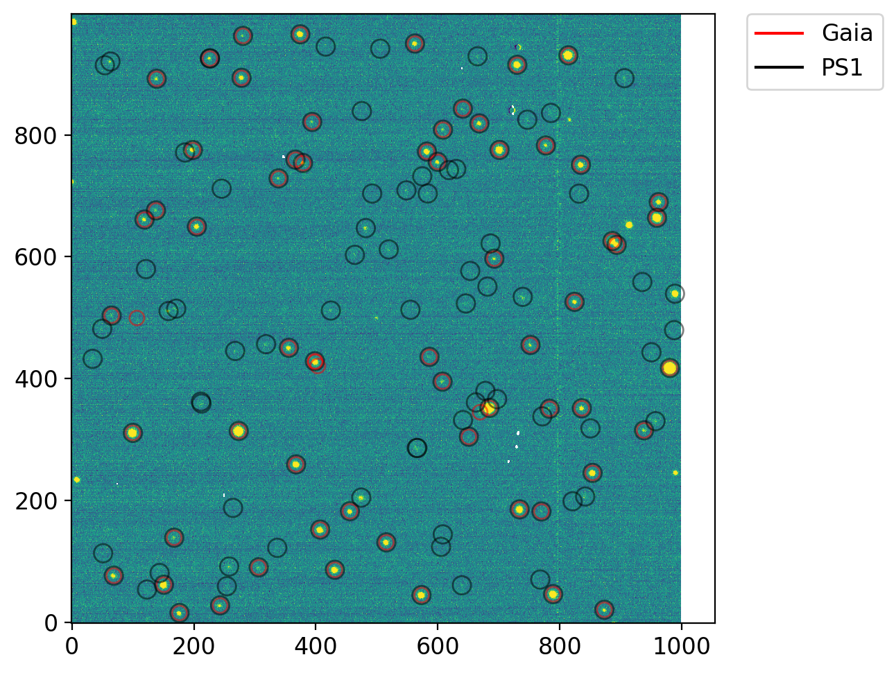
aps1 = CircularAperture(np.array([q1["x"], q1["y"]]).T, r=12)
aps2 = CircularAperture(np.array([q2["x"], q2["y"]]).T, r=15)

fig, axs = plt.subplots(1, 1, figsize=(8, 5), sharex=False, sharey=False, gridspec_kw=None)

vis.norm_imshow(axs, ccd, zscale=True)
aps1.plot(color='r', lw=1, alpha=0.5, ax=axs)
aps2.plot(color='k', lw=1, alpha=0.5, ax=axs)

for c, l in zip("rk", ["Gaia", "PS1"]):
    axs.plot(np.nan, np.nan, f"{c}", label=l)
axs.legend(bbox_to_anchor=(1.05, 1), loc='upper left', borderaxespad=0.)

plt.tight_layout()
plt.show();

5.3.4. A Short Discussion

Note that there are more objects in PS1 than Gaia. Since Gaia’s main purpose is astrometry, it is not surprising that PS1 is sensing more celestial objects. Also, PS1 has the filter system that is closer to the classical filter systems (it uses grizy). Thus, for ground-based differential photometry, PS1 catalog will be more useful.

5.4. JPL HORIZONS (Solar System)

JPL HORIZONS is a ephemeris (plural ephemerides) service operated by NASA JPL. The main purpose of this tool is to perform precise N-body simulation, including the modern computational algorithms, and provide the results to the users. There are many cases you may need it, but the main purpose is to obtain the positional information of the solar system objects or satellite or spacecrafts at certain epoch(s).

Practice

For example, let’s query the information of our target in the CCD image that we are using. We took the image of asteroid (4179) Toutatis on UT 2018-04-13T21:30 (see ccd.header["DATE-OBS"]).

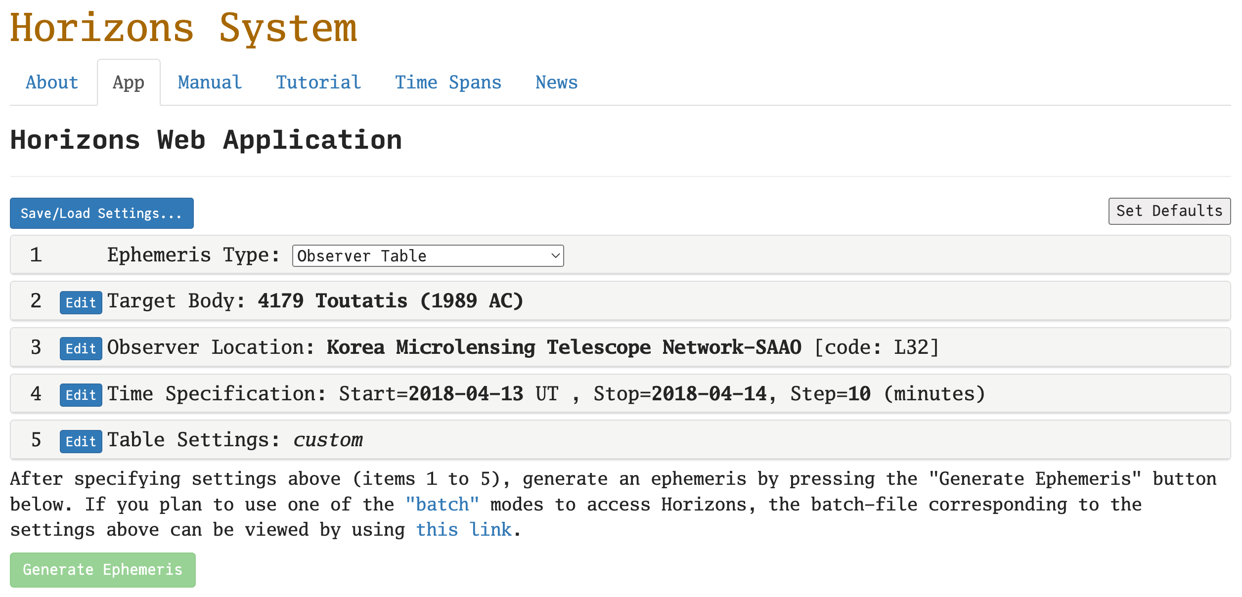
Set the table as below:

1. Ephemeris Type: "Observer Table"

2. Target Body: Click edit and search for 4179.

3. Observer Location: Search for SAAO and select Korea Microlensing Telescope Network-SAAO (code: L32)

4. Time Specification: Insert start/stop times as 2018-04-13 and 2018-04-14. Type Step size of 10 and "minutes".

5. Table Settings: Click edit and select "Default" button.

   • “Additional Table Settings”: Elevation cutoff: 10, check the box of “Skip daylight”

Then hit the “Generate Ephemeris” button. You will see a long output, but what’s important is just the lines near the observation time (UT 2018-04-13T21:30):

Date__(UT)__HR:MN     R.A._____(ICRF)_____DEC    APmag   S-brt             delta      deldot     S-O-T /r     S-T-O  Sky_motion  Sky_mot_PA  RelVel-ANG  Lun_Sky_Brt  sky_SNR
2018-Apr-13 22:30     13 37 24.57 -09 29 35.4   20.609   7.453  2.82285755430415   2.9894066  177.5789 /L    0.6391   0.5987445   290.83331   8.3188634         n.a.     n.a.

The explanation for each column is given at the bottom of the website. Important ones are the time (Date__(UT)__HR:MN), RA/DEC (R.A._____(ICRF)_____DEC), and the expected V-band magnitude (APmag). Sometimes you may need the heliocentric and geocentric distances (go to the Table Settings and check number 19 & 20).

After generating the ephemerides, you can see the detailed explanations of each column at the bottom part of the result page. https://astroquery.readthedocs.io/en/latest/jplhorizons/jplhorizons.html

From python, you can access HORIZONS using astroquery’s JPLHorizons module, thanks to M. Mommert:

objname = "4179"
observat = "L32"
t_obs = Time(ccd.header["DATE-OBS"]) + ccd.header["EXPTIME"] * u.s / 2
obj = Horizons(id=objname, location=observat, epochs=t_obs.jd)
obj_q = obj.ephemerides()
obj_q.pprint(max_width=100)

       targetname             datetime_str          datetime_jd    ... alpha_true  PABLon  PABLat
          ---                     ---                    d         ...    deg       deg     deg  
----------------------- ------------------------ ----------------- ... ---------- -------- ------
4179 Toutatis (1989 AC) 2018-Apr-13 21:30:56.000 2458222.396481481 ...     0.6463 205.7217 0.5207

The resulting obj_q contains many columns and they have slightly different names than that of HORIZONS you saw above. They are summarized in the official documentation. Few important columns are

• RA and DEC: The RA/DEC in degrees.

• lighttime: asteroid-observer distance / c = time delay. The true time of light when it departed the object is, thus, observed time - lighttime.

• alpha: The phase angle in degrees (alpha differ from alpha_true by only less than around 1 arcmin, so astronomers just use alpha, not alpha_true).

Practice

What if observatory has no designated code (e.g., SNU observatory)?

The answer is clearly written in the documentation. For SNU bldg 45 and 46, you can use location=dict(lon=126.95, lat=37.45, elevation=0.1).

Note

In real work, you don’t want to query this for every image (as it takes a lot of time). Better way is to obtain the t_obs for all the images and pass that as Horizons(..., epochs=t_obs_list) as python list object. See the official documentation for the usage, if necessary.

Once we know the RA/DEC, we can convert those to the image XY coordinate by using the WCS information in the header, as we did for stars:

pos_sky = SkyCoord(obj_q["RA"][0], obj_q["DEC"][0], unit='deg')
pos_pix = pos_sky.to_pixel(wcs=ccd.wcs)
print(pos_sky)
print(pos_pix)

ap0 = CircularAperture(np.array([pos_pix[0], pos_pix[1]]).T, r=20)

fig, axs = plt.subplots(1, 1, figsize=(8, 5), sharex=False, sharey=False, gridspec_kw=None)

vis.norm_imshow(axs, ccd, zscale=True)
aps2.plot(color='k', lw=1, alpha=0.5, ax=axs)
ap0.plot(color='r', lw=1, alpha=1, ax=axs)

plt.tight_layout()
plt.show();

<SkyCoord (ICRS): (ra, dec) in deg
    (204.36166, -9.49665)>
(array(500.58291238), array(500.43561473))

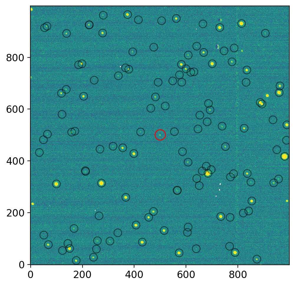
The red circle is the location of our asteoid, (4179) Toutatis.