Isophote fitting: ELLIPSE analysis

Purpose of this tutorial

We show the capability of aap photometry when ellipses are given. This includes
- growth curve,
- surface brightness between isophotes,
- mask handling.
Ellipse (isophote) fitting is not the purpose of aap. We use photutils.isophote for the fitting, and the fitting algorithm is not reproduced in this notebook.

photutils.isophote fitting will follow the Jedrzejewski (1987) method, as IRAF ellipse.

Isophote: curve of constant surface brightness. For most elliptical galaxies and bulges, each isophote is close to an ellipse.

The radial dependence of shape is often of interest:

Ellipticity \(\varepsilon(a) = 1 - b/a\) may indicate dynamics and/or inclination.
Position angle \(\theta(a)\) shows isophote twists, which may indicate triaxiality, a bar, or multiple components with different orientations.
The fourth harmonic \(b_4(a)\) shows disky (\(b_4 > 0\)) or boxy (\(b_4 < 0\)) isophotes (a classic diagnostic for elliptical galaxies).
Surface brightness \(\mu(a)\) along the isophotes is the input for Sérsic or bulge/disk profile fits.

We fit the isophotes with (1) photutils.isophote (the astropy affiliated tool), then (2) show how astroapers can be used for further analyses:

Surface brightness between isophotes: EllipAn with the inner and outer ellipses (two differently shaped ellipses can define an annulus in aap) using exact flux and area. Masked pixels (e.g., a foreground star or SNe, cosmic-ray, satellite streak, solar system objects, etc) are excluded (mask=).
Curve of growth: Make EllipAp for each isophote (exact pixel overlap), do photometry and see how it changes over radius. Masked pixels are filled with a representative value of each annulus (item 1).

import matplotlib.pyplot as plt
import numpy as np
import photutils
from astropy.modeling import fitting
from astropy.modeling.models import Gaussian2D, Sersic1D
from photutils.isophote import Ellipse, EllipseGeometry

import astroapers as aap

print(f"photutils {photutils.__version__}")

photutils 3.0.0

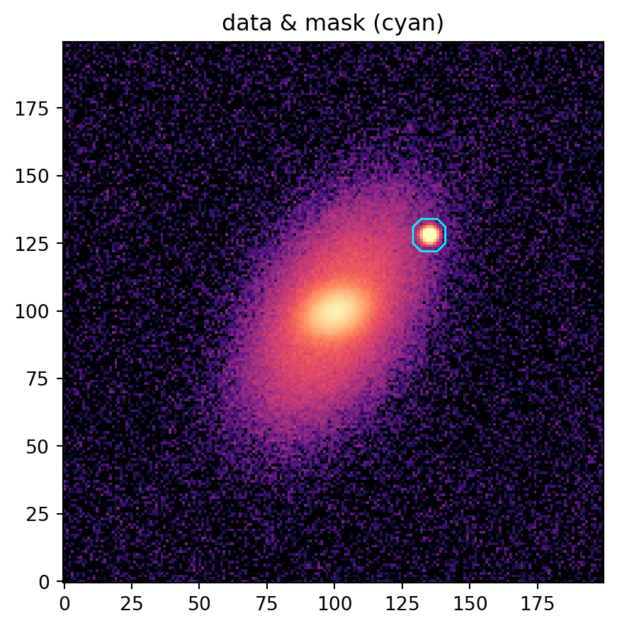
A synthetic galaxy

Two elliptical Gaussians (Gaussian2D, as in the photutils.isophote example docs), so that \(\varepsilon\) and \(\theta\) change with radius:

Inner = amplitude 100, \(\sigma\) = 7 × 5 pix (\(\varepsilon = 0.29\)), \(\theta = 20°\)
Outer = amplitude 30, \(\sigma\) = 28 × 16 pix (\(\varepsilon = 0.43\)), \(\theta = 60°\)

plus Gaussian noise (\(\sigma = 2\)) and a bright star, which is masked.

ny = nx = 200
XCEN, YCEN = 100.3, 99.6
yy, xx = np.mgrid[:ny, :nx]

inner = Gaussian2D(
    100.0, XCEN, YCEN, x_stddev=7.0, y_stddev=5.0, theta=np.deg2rad(20)
)
outer = Gaussian2D(
    30.0, XCEN, YCEN, x_stddev=28.0, y_stddev=16.0, theta=np.deg2rad(60)
)
galaxy = inner(xx, yy) + outer(xx, yy)  # noiseless truth

# Add a bright star
star_x, star_y = 135.0, 128.0
star = Gaussian2D(500.0, star_x, star_y, x_stddev=1.5, y_stddev=1.5)
mask = np.hypot(xx - star_x, yy - star_y) < 6.0  # True = excluded

rng = np.random.default_rng(0)

# simulate data with random noise addition
data = galaxy + star(xx, yy) + rng.normal(0.0, 2.0, galaxy.shape)

fig, ax = plt.subplots(1, 1, figsize=(9, 4.5), sharex=True, sharey=True, constrained_layout=True)
ax.imshow(np.arcsinh(data / 2), origin="lower", cmap="magma", vmin=0, vmax=5)
# masked = 1, unmasked =0
ax.contour(mask, levels=[0.01], colors="cyan", linewidths=1)
ax.set_title("data & mask (cyan)")
plt.show()

`photutils`: Fit Isophotes

Using photutils first.

First with a free center. Then second, fix the center at the median (outer, noisy isophotes let the free center wander; a fixed center also lets the EllipAn annuli below share one position).

masked = np.ma.array(data, mask=mask)

# start with initial guess
guess = EllipseGeometry(x0=100.0, y0=100.0, sma=10.0, eps=0.3, pa=np.deg2rad(30))

# Initiate photutils Ellipse (free center == photutils default)
free = Ellipse(masked, geometry=guess).fit_image(minsma=2.0)
x_c, y_c = np.median(free.x0), np.median(free.y0)

# Refit with the center fixed (our choice, not a photutils default)
guess = EllipseGeometry(x0=x_c, y0=y_c, sma=10.0, eps=0.3, pa=np.deg2rad(30))
isolist = Ellipse(masked, geometry=guess).fit_image(minsma=2.0, fix_center=True)  # skip a < 2 pix
print(f"center: ({x_c:.2f}, {y_c:.2f})   true: ({XCEN}, {YCEN});   {len(isolist)} isophotes")

# IsophoteList.to_table() -> astropy QTable (every 5th row shown)
tab = isolist.to_table()["sma", "intens", "ellipticity", "ellipticity_err", "pa", "pa_err", "stop_code"][::5]
tab.round(3)
tab

center: (100.33, 99.58)   true: (100.3, 99.6);   40 isophotes

DeprecatedColumnQTable length=8

sma	intens	ellipticity	ellipticity_err	pa	pa_err	stop_code
				deg	deg
float64	float64	float64	float64	float64	float64	int64
2.176	124.452	0.271	0.029	25.453	3.614	0
3.505	117.203	0.266	0.02	15.543	2.583	0
5.645	100.617	0.287	0.008	21.376	0.996	0
9.091	69.945	0.269	0.005	22.703	0.636	0
14.641	35.165	0.254	0.007	29.102	0.867	0
23.579	20.979	0.336	0.012	53.796	1.205	0
37.975	11.61	0.425	0.01	59.678	0.908	2
61.159	2.722	0.422	0.013	59.606	1.165	2

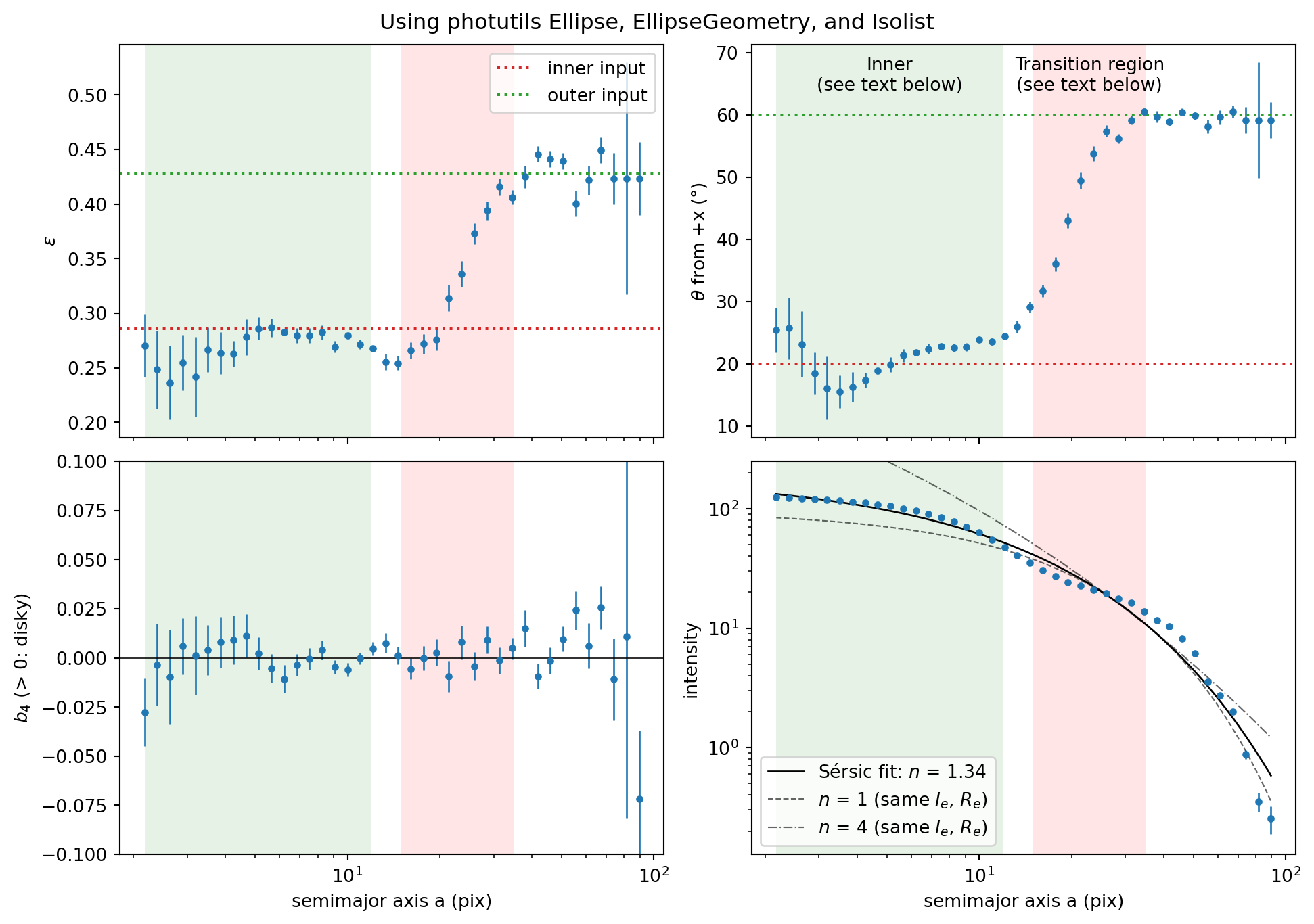
Now draw ellipticity, PA, B4, and intensity (radial profile).

For the intensity, we fit the Sérsic law (astropy.modeling.models.Sersic1D), the standard power law in the exponent:

\[ I(a) = I_e \exp\left\{ -b(n) \left[ \left( \frac{a}{R_e} \right)^{1/n} - 1 \right] \right\} \]

\(a\) is semimajor axis (isophote), \(R_e\) os effective (half-light) radius along \(a\), and \(I_e = I(R_e)\).
\(n\) = Sérsic index.
- \(n = 0.5\): Gaussian
- \(n = 1\): exponential (disk)
- \(n = 4\): de Vaucouleurs (ellipticals, classical bulges)
\(b(n)\) is a parameter such that \(R_e\) encloses half the light

# Sérsic fit, weighted by the photutils intensity errors
init = Sersic1D(
    amplitude=np.interp(20, isolist.sma, isolist.intens), r_eff=20.0, n=1.0
)

sersic = fitting.TRFLSQFitter()(
    init, isolist.sma, isolist.intens, weights=1 / isolist.int_err
)

print(f"Sérsic: I_e = {sersic.amplitude.value:.1f}, R_e = {sersic.r_eff.value:.1f} pix, n = {sersic.n.value:.2f}")

fig, axes = plt.subplots(2, 2, figsize=(10, 7), sharex=True, constrained_layout=True)
kw = dict(fmt="o", ms=3, elinewidth=1)
axes[0, 0].errorbar(isolist.sma, isolist.eps, isolist.ellip_err, **kw)
axes[0, 1].errorbar(isolist.sma, np.rad2deg(isolist.pa), np.rad2deg(isolist.pa_err), **kw)
axes[1, 0].errorbar(isolist.sma, isolist.b4, isolist.b4_err, **kw)
axes[1, 1].errorbar(isolist.sma, isolist.intens, isolist.int_err, **kw)

# Input values of the two Gaussians
for ax, (v_in, v_out) in zip(axes[0], [(1 - 5/7, 1 - 16/28), (20, 60)]):
    ax.axhline(v_in, color="C3", ls=":", label="inner input")
    ax.axhline(v_out, color="C2", ls=":", label="outer input")

# Inner and transition regions (see text below)
for ax in axes.flat:
    ax.axvspan(isolist.sma[0], 12, color="g", alpha=0.1, lw=0)
    ax.axvspan(15, 35, color="r", alpha=0.1, lw=0)
for x, name in [(np.sqrt(isolist.sma[0] * 12), "Inner"), (np.sqrt(15 * 35), "Transition region")]:
    axes[0, 1].text(
        x, 0.97, f"{name}\n(see text below)", 
        transform=axes[0, 1].get_xaxis_transform(),
        ha="center", va="top"
    )

# Sérsic fit, and typical n = 1 and 4 with the same I_e and R_e
a_grid = np.geomspace(isolist.sma[0], isolist.sma[-1], 200)
axes[1, 1].plot(a_grid, sersic(a_grid), "k-", lw=1, label=f"Sérsic fit: $n$ = {sersic.n.value:.2f}")
for n, ls in [(1, "--"), (4, "-.")]:
    ref = Sersic1D(sersic.amplitude, sersic.r_eff, n)
    axes[1, 1].plot(
        a_grid, ref(a_grid), "k", ls=ls, lw=0.8, alpha=0.6, 
        label=f"$n$ = {n} (same $I_e$, $R_e$)"
    )
axes[1, 1].set_ylim(0.5 * isolist.intens.min(), 2 * isolist.intens.max())

axes[0, 0].legend()
axes[1, 1].legend()
axes[1, 0].axhline(0, color="k", lw=0.6)
axes[1, 0].set_ylim(-0.1, 0.1)
axes[1, 1].set_yscale("log")
labels = [r"$ε$", r"$θ$ from +x (°)", r"$b_4$ (> 0: disky)", "intensity"]
for ax, label in zip(axes.flat, labels):
    ax.set(xscale="log", ylabel=label)
for ax in axes[1]:
    ax.set_xlabel("semimajor axis a (pix)")
fig.suptitle("Using photutils Ellipse, EllipseGeometry, and Isolist")
plt.show()

Sérsic: I_e = 18.0, R_e = 26.8 pix, n = 1.34

Inner (\(a \lesssim 12\) pix): approximately inner input \((\varepsilon, \theta) = (0.29, 20°)\).
Transition region (\(15 \lesssim a \lesssim 35\) pix).
\(b_4 \approx 0\) (within \(2\sigma\)): no disky/boxy isophotes, as in the input.
Intensity: We used 2 Gaussians (each == \(n = 0.5\)) are not one Sérsic.

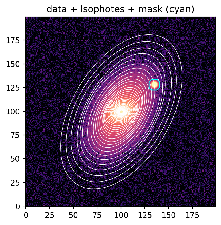
The ellipses from photutils:

# outputs from photutils
sma = isolist.sma
b_ax = sma * (1 - isolist.eps)  # semiminor axes
pa = isolist.pa

fig, ax = plt.subplots(figsize=(5, 4.5))
ax.imshow(np.arcsinh(data / 2), origin="lower", cmap="magma", vmin=0, vmax=5)
ax.contour(mask, levels=[0.5], colors="cyan", linewidths=1)

# Draw isophotes (plotter within aap)
for a, b, t in zip(sma, b_ax, pa):
    aap.EllipAp((x_c, y_c), a, b, t).plot(ax=ax, color="w", lw=0.6)
ax.set_title("data + isophotes + mask (cyan)")
plt.show()

`astroapers`: Photometry

aap part starts from the ellipses (center, \(a\), \(b = a(1 - \varepsilon)\), \(\theta\)).

We use output from photutils here, but any source works (your own fit, literature values, …).

Between isophotes (`EllipAn`)

One can do a simple naive photometry: From the ellipses (isophots) from photutils, use i-th and i+1-th ellipses as inner and outer boundaries to make an elliptical annulus.

annuli = [
    aap.EllipAn((x_c, y_c), a_in=a0, b_in=b0, a_out=a1, b_out=b1, theta_in=t0, theta_out=t1)
    for a0, b0, t0, a1, b1, t1 
    in zip(sma[:-1], b_ax[:-1], pa[:-1], sma[1:], b_ax[1:], pa[1:])
]
ann_flux, ann_npix = np.array(
    [an.apsum_exact(data, mask=mask) for an in annuli]
).T
# npix is the effective area 'excluding' masked pixels or pixels outside image.
ann_mean = ann_flux / ann_npix

# analytic area (incl. masked pixels); will be used later for the curve of growth:
ann_area = np.array([an.area for an in annuli])

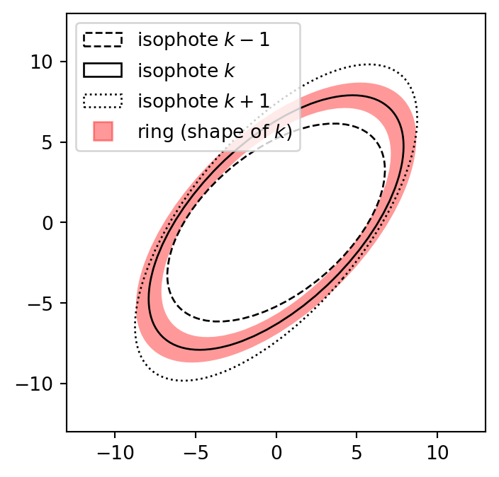
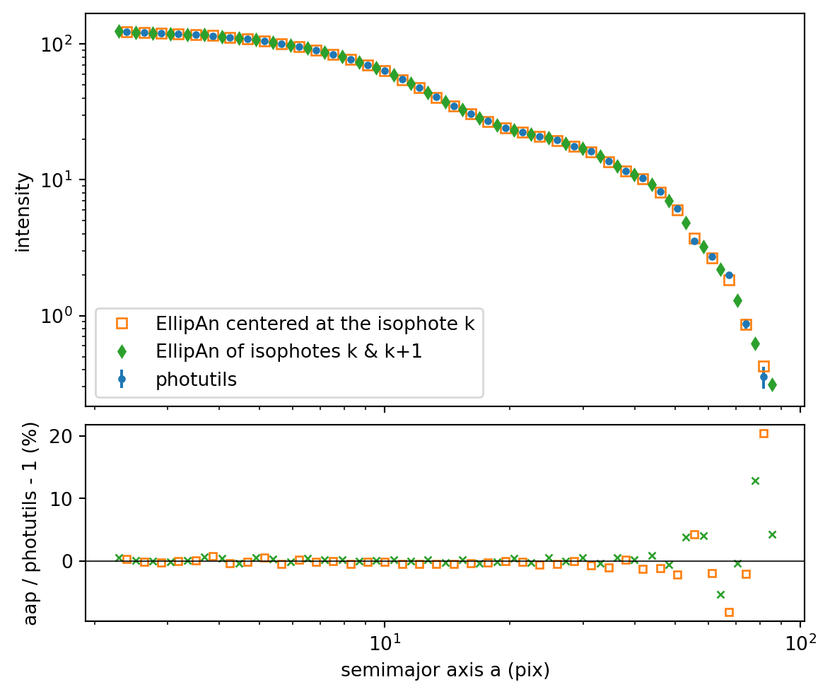
But to compare with photutils (intensity along isophote \(k\)), make a thin ring around isophote \(k\):

Use \(\varepsilon_k\), \(\theta_k\) (shape identical to the isophote \(k\))
\(a_\mathrm{in} = (a_{k-1} + a_k)/2\)
\(a_\mathrm{out} = (a_k + a_{k+1})/2\)

Below is a schematic diagram:

# Schematic diagram with made-up ellipses: isophotes k-1, k, k+1
a_s = np.array([8.0, 10.0, 12.0])
q_s = 1 - np.array([0.45, 0.50, 0.55])  # axis ratio b/a
t_s = np.deg2rad([40.0, 45.0, 50.0])
a_in, a_out = (a_s[0] + a_s[1]) / 2, (a_s[1] + a_s[2]) / 2  # 9 and 11

fig, ax = plt.subplots(figsize=(4, 4))
an_draw = aap.EllipAn(
    (0, 0), 
    a_in=a_in, b_in=a_in * q_s[1], 
    a_out=a_out, b_out=a_out * q_s[1], 
    theta_in=t_s[1], theta_out=t_s[1]
)
an_draw.plot(ax=ax, fill=True, facecolor="r", alpha=0.4, lw=0)
for a, qq, tt, ls, label in zip(a_s, q_s, t_s, ["--", "-", ":"], ["isophote $k-1$", "isophote $k$", "isophote $k+1$"]):
    aap.EllipAp((0, 0), a, a * qq, tt).plot(ax=ax, color="k", ls=ls, lw=1, label=label)
ax.plot([], [], "rs", alpha=0.4, ms=10, label="ring (shape of $k$)")
ax.set(xlim=(-13, 13), ylim=(-13, 13), aspect="equal")
ax.legend(loc="upper left")
plt.show()

Now, do that for our data:

a_mid = (sma[:-1] + sma[1:]) / 2  # midpoints between consecutive isophotes
q = 1 - isolist.eps               # axis ratio b/a

# annulus *around* the k-th isophote (k = 1, ..., N-2), with its own shape
around = [
    aap.EllipAn(
        (x_c, y_c), 
        a_in=a0, b_in=a0*qk, 
        a_out=a1, b_out=a1*qk, 
        theta_in=tk, theta_out=tk
    ) for a0, a1, qk, tk in zip(a_mid[:-1], a_mid[1:], q[1:-1], pa[1:-1])
]

flux, npix = np.array([an.apsum_exact(data, mask=mask) for an in around]).T
around_mean = flux / npix
sma_k, I_phot = sma[1:-1], isolist.intens[1:-1]

fig, axes = plt.subplots(2, 1, figsize=(6, 5), sharex=True, height_ratios=[2, 1], constrained_layout=True)

_l = axes[0].errorbar(
    sma_k, I_phot, isolist.int_err[1:-1], fmt="o", ms=3, label="photutils"
)
_l_ring = axes[0].plot(
    sma_k, around_mean, "s", ms=5, mfc="none", label="EllipAn centered at the isophote k"
)
_l_naive = axes[0].plot(
    a_mid, ann_mean, "d", ms=4, label="EllipAn of isophotes k & k+1"
)
axes[0].set(yscale="log", ylabel="intensity")
axes[0].legend()
axes[1].plot(sma_k, 100 * (around_mean / I_phot - 1), "s", ms=4, mfc="none", color=_l_ring[0].get_color())

# naive: photutils intensity interpolated (log-log) to the midpoint a
ann_mean_photutils_interp = np.exp(
    np.interp(np.log(a_mid), np.log(sma), np.log(isolist.intens))
)
axes[1].plot(
    a_mid, 100 * (ann_mean / ann_mean_photutils_interp - 1), 
    "x", ms=4, color=_l_naive[0].get_color()
)
axes[1].axhline(0, color="k", lw=0.6)
axes[1].set(xscale="log", xlabel="semimajor axis a (pix)", ylabel="aap / photutils - 1 (%)")
plt.show()

aap and photutils match within ~1% for \(a < 50\) pix (bottom panel).

Why two differ above (different computations):

photutils’s intens is mean of points on the ellipse line (~1 pix apart), by bilinear interpolation from the 4 nearest pixels.
In our aap, it did area-weighted mean of all pixels within the EllipAn with width ~10% of \(a\).

Curve of growth (`EllipAp`)

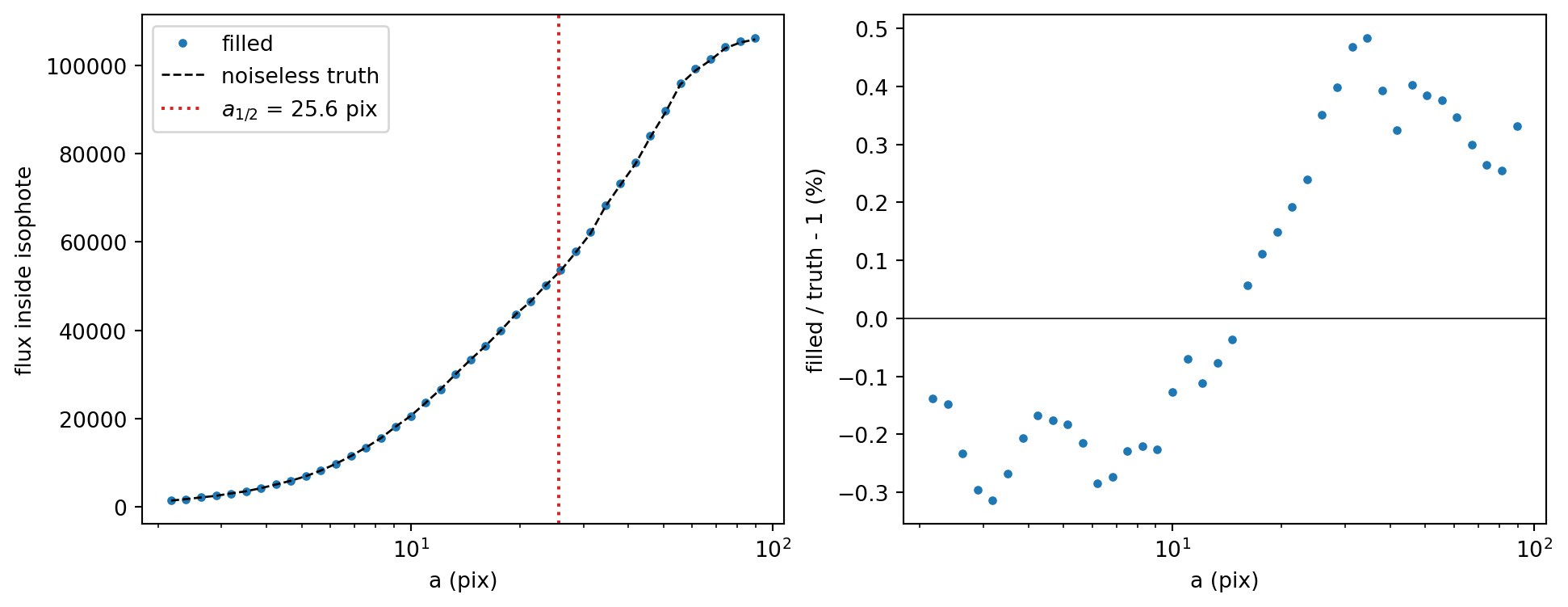
Curve of growth (cog below) is flux inside each isophote vs. \(a\), with the masked part of each annulus filled by a representative value of that annulus:

\[ F_k = F_0 + \sum_{j=0}^{k-1} \left[ S_j + I_j (A_j - n_j) \right] \]

Numbering (same as the Python indices):
- Isophote \(k = 0, 1, \dots\) from the innermost (sma[k]).
- Annulus \(j\) = the naive EllipAn between isophotes \(j\) and \(j+1\) (annuli[j], above).
\(F_k\) = flux inside isophote \(k\) (cog[k]).
- \(F_0\) = flux inside the innermost isophote (f0). It has no masked pixels here.
\(S_j\) = measured flux of annulus \(j\), masked pixels excluded (ann_flux[j]).
\(n_j\) = effective area (i.e., masked pixels excluded) of annulus \(j\) (ann_npix[j]); \(A_j\) = its analytic area (i.e., total area; ann_area[j]).
- So \(A_j - n_j\) = its masked area.
\(I_j\) = representative value of annulus \(j\), used only for its masked area.
- Here: area-weighted mean, \(I_j = S_j / n_j\) (ann_mean[j]). Then \(S_j + I_j (A_j - n_j) = I_j A_j\).
- Median, mode, sigma-clipped mean, … also work, e.g., np.median(annuli[j].sampled_values(data, mask=mask)[0]).

ap0 = aap.EllipAp((x_c, y_c), sma[0], b_ax[0], pa[0])
f0 = ap0.apsum_exact(data, mask=mask, return_npix=False)
cog = f0 + np.concatenate([[0], np.cumsum(ann_flux + ann_mean * (ann_area - ann_npix))])  # curve of growth: cog[k] = F_k
cog_true = np.array([
    aap.EllipAp((x_c, y_c), a, b, t).apsum_exact(galaxy, return_npix=False)
    for a, b, t in zip(sma, b_ax, pa)
])

# Check: filled flux in the masked pixels vs. the noiseless truth there
fill = np.sum((ann_area - ann_npix) * ann_mean)
print(f"masked pixels: {mask.sum()};  filled flux = {fill:.0f}, truth = {galaxy[mask].sum():.0f}")

# Half-light semimajor axis (of the light inside the last isophote)
a_half = np.interp(0.5 * cog[-1], cog, sma)
print(f"a_half = {a_half:.1f} pix")

fig, axes = plt.subplots(1, 2, figsize=(10, 3.8), constrained_layout=True)
axes[0].plot(sma, cog, "o", ms=3, label="filled")
axes[0].plot(sma, cog_true, "k--", lw=1, label="noiseless truth")
axes[0].axvline(a_half, color="C3", ls=":", label=f"$a_{{1/2}}$ = {a_half:.1f} pix")
axes[0].set(xscale="log", xlabel="a (pix)", ylabel="flux inside isophote")
axes[0].legend()
axes[1].plot(sma, 100 * (cog / cog_true - 1), "o", ms=3)
axes[1].axhline(0, color="k", lw=0.6)
axes[1].set(xscale="log", xlabel="a (pix)", ylabel="filled / truth - 1 (%)")
plt.show()

masked pixels: 109;  filled flux = 669, truth = 656
a_half = 25.6 pix

Right: the difference ≈ pixel noise inside each ellipse.

Notes

\(\theta\) (pa in photutils) is from the image \(+x\) axis toward \(+y\) (counterclockwise).
- Sky PA (north through east) depends on the WCS, e.g., north up & east left: PA = \(\theta - 90°\).
Be careful in extreme cases when \(k\) and \(k+1\) isophotes actually cross each other. That’s when astronomer’s decision must happen.
\(a_{1/2}\) above is half of the light inside the last isophote, not the total light.

A synthetic galaxy

photutils: Fit Isophotes

astroapers: Photometry

Between isophotes (EllipAn)

Curve of growth (EllipAp)

Notes

`photutils`: Fit Isophotes

`astroapers`: Photometry

Between isophotes (`EllipAn`)

Curve of growth (`EllipAp`)