Multiple apertures and radial profiles

This notebook shows how to measure several source positions at once, check edge coverage, and use multiple radii to build a simple radial profile.

import numpy as np
import matplotlib.pyplot as plt
import astroapers as aap
import pandas as pd

Several apertures at once

ny, nx = 70, 80
y, x = np.mgrid[:ny, :nx]
positions = np.array(
    [
        [20.0, 24.0],
        [40.5, 35.2],
        [78.0, 68.0],
    ],
)

data = np.full((ny, nx), 5.0)
for x0, y0 in positions:
    data += 80.0 * np.exp(-0.5 * ((x - x0) ** 2 + (y - y0) ** 2) / 2.5**2)

# multiple apertures at once:
ap = aap.CircAp(positions, r=5.0)

# all at once:
apsum, npix = ap.apsum_exact(data)
coverage = npix / ap.area

assert coverage[-1] < 1.0
pd.DataFrame({
    "x": positions[:, 0],
    "y": positions[:, 1],
    "apsum": apsum,
    "npix": npix,
    "coverage": coverage
})

	x	y	apsum	npix	coverage
0	20.0	24.0	3095.883704	78.539816	1.000000
1	40.5	35.2	3098.910513	78.539816	1.000000
2	78.0	68.0	1697.748072	36.656814	0.466729

The third source is near the image edge, so its in-frame coverage is smaller.

fig, ax = plt.subplots(figsize=(5, 4))
ax.imshow(data, origin="lower", cmap="viridis")
ap.plot(ax=ax, color="r", lw=2)
ax.set_title("Multiple circular apertures")
plt.show()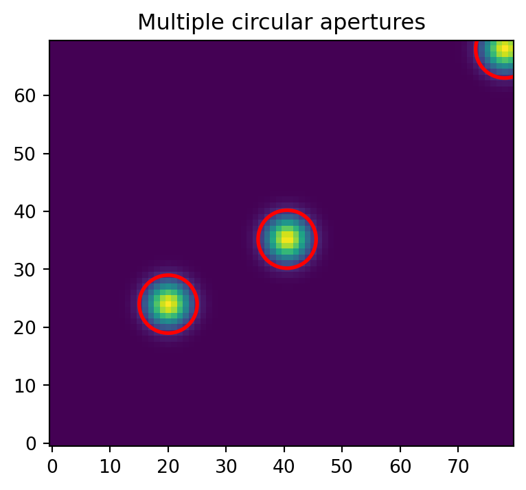

Multiple radii for radial profiles

Use one vector aperture per radius to measure the same source catalog at several scales. The examples below use the two in-frame sources; the edge source is excluded so the radial profile is not dominated by image clipping.

# drop objects with low coverage:
edgemask = npix < ap.area

profile_positions = positions[~edgemask]
radii = np.arange(1.0, 10.0, 1.0)

cumulative = []
for radius in radii:
    ap_r = aap.CircAp(profile_positions, r=radius)
    ap_r_sum, ap_r_npix = ap_r.apsum_exact(data)
    cumulative.append((ap_r_sum, ap_r_npix))

cumulative_apsum = np.vstack([row[0] for row in cumulative])
cumulative_npix = np.vstack([row[1] for row in cumulative])

pd.DataFrame(
    cumulative_apsum,
    index=pd.Index(radii, name="radius"),
    columns=[f"source {idx}" for idx in range(len(profile_positions))],
)

	source 0	source 1
radius
1.0	252.073757	255.234593
2.0	909.846200	915.437406
3.0	1734.940312	1741.407368
4.0	2501.349863	2506.335847
5.0	3095.883704	3098.910513
6.0	3522.928796	3524.545542
7.0	3845.326896	3845.881803
8.0	4126.672944	4126.909342
9.0	4408.660903	4408.716454

Draw the same radii on the image:

fig, ax = plt.subplots(figsize=(5, 4))
ax.imshow(data, origin="lower", cmap="viridis")
for radius in radii:
    aap.CircAp(profile_positions, r=radius).plot(
        ax=ax,
        color="tab:red",
        alpha=0.35,
        lw=1.2,
    )
ax.scatter(profile_positions[:, 0], profile_positions[:, 1], c="white", s=12)
ax.set_title("Multiple radii at each source")
plt.show()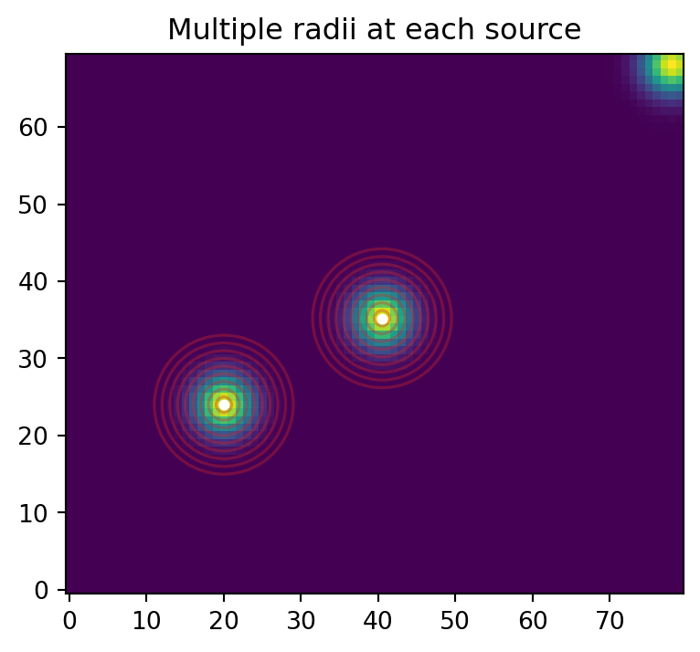

For custom pixel-sample statistics such as a sigma-clipped median, or robust scatter, each aperture returns a different number of raw image values. That result is ragged, so a Python reduction over the returned arrays is expected. Keep the aperture construction vectorized over source positions, and use the length of each returned sample array as the center-selected pixel count. Use weights_center() instead when you need the bbox-tight binary weights themselves.

radius_edges = np.arange(0.0, 10.0, 1.0)
radius_mid = 0.5 * (radius_edges[:-1] + radius_edges[1:])

custom_rows = []
for r_in, r_out, r_mid in zip(radius_edges[:-1], radius_edges[1:], radius_mid):
    an = aap.CircAn(profile_positions, r_in=r_in, r_out=r_out)
    an_vals = an.sampled_values(data)

    # For raw center-selected samples, npix is just the number of values used here.
    # For complicated calculations, user may store npix before/after sigclip
    # such as npix and nrej.

    for source_idx, ((x0, y0), vals) in enumerate(zip(profile_positions, an_vals)):
        custom_rows.append(
            {
                "radius": r_mid,
                "source": source_idx,
                "x": x0,
                "y": y0,
                "mpix": np.nanmedian(vals),
                "spix": np.nanstd(vals, ddof=1),
                "npix": len(vals),
            }
        )

custom_profile = pd.DataFrame(custom_rows).set_index(["radius", "source"])
custom_profile

		x	y	mpix	spix	npix
radius	source
0.5	0	20.0	24.0	85.000000	NaN	1
0.5	1	40.5	35.2	81.333707	2.115016	4
1.5	0	20.0	24.0	76.010405	3.034914	8
1.5	1	40.5	35.2	68.486459	4.045531	10
2.5	0	20.0	24.0	58.625604	6.081807	16
2.5	1	40.5	35.2	51.100631	4.026071	14
3.5	0	20.0	24.0	40.946317	4.498758	20
3.5	1	40.5	35.2	34.453909	4.594058	22
4.5	0	20.0	24.0	24.743541	2.336489	24
4.5	1	40.5	35.2	20.532811	3.229756	28
5.5	0	20.0	24.0	13.928152	2.213032	40
5.5	1	40.5	35.2	11.978449	1.912151	38
6.5	0	20.0	24.0	8.260976	0.792907	36
6.5	1	40.5	35.2	7.466881	0.713340	40
7.5	0	20.0	24.0	6.200606	0.342251	48
7.5	1	40.5	35.2	5.831067	0.276280	44
8.5	0	20.0	24.0	5.299624	0.119430	56
8.5	1	40.5	35.2	5.232901	0.106322	56

For high-throughput grouped statistics, flat=True returns the same ragged samples as one concatenated array plus integer offsets. Aperture i is flat_values[offsets[i]:offsets[i + 1]], and np.split() reconstructs the default list result.

flat_values, offsets = an.sampled_values(data, flat=True)
assert all(
    np.array_equal(got, want)
    for got, want in zip(np.split(flat_values, offsets[1:-1]), an_vals)
)

flat_values.shape, offsets.shape

((112,), (3,))

fig, ax = plt.subplots(figsize=(5, 3.5))
for source_idx, source_profile in custom_profile.groupby(level="source"):
    x0 = source_profile["x"].iloc[0]
    y0 = source_profile["y"].iloc[0]

    # Median surface brightness (divide by area), normalized by the central annulus:
    sample_npix = source_profile["npix"]
    surf_b = source_profile["mpix"] / sample_npix
    center = surf_b.iloc[0]
    surf_b = surf_b / center
    spix_surfb = source_profile["spix"] / center / sample_npix

    ax.errorbar(
        source_profile.index.get_level_values("radius"),
        surf_b,
        yerr=spix_surfb,
        marker=".",
        label=f"({x0:.1f}, {y0:.1f})",
    )
ax.legend(title="source")
ax.set(
    xlabel="radius (pixels)",
    ylabel="Surface brightness (normalized)",
    yscale="log",
)
plt.show()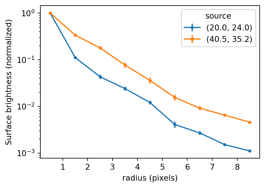

Weights and boxes return lists

weights_exact() and bboxes() each return one item per vector position, even when the aperture is scalar. Match them by index when clipping or reusing bbox-tight weights.

weights = ap.weights_center()
boxes = ap.bboxes()
assert len(weights) == len(positions)
[weight.sum() for weight in weights]

[np.float64(69.0), np.float64(78.0), np.float64(69.0)]

full_masks = [
    box.to_image(weight, data.shape) > 0
    for weight, box in zip(weights, boxes, strict=True)
]
[mask.sum() for mask in full_masks]

[np.int64(69), np.int64(78), np.int64(33)]

Maximum Performance

For catalog arrays, import the raw Rust extension as aapr. Keep x, y, and data contiguous, and pass geometry as positional arguments. For more examples of raw call patterns, inspect astroapers.kernels.

import astroapers._rust as aapr

raw_data = np.ascontiguousarray(data, dtype=np.float64)
xpos = np.ascontiguousarray(positions[:, 0], dtype=np.float64)
ypos = np.ascontiguousarray(positions[:, 1], dtype=np.float64)

raw_apsum, raw_npix = aapr.apsum_circ_exact(raw_data, xpos, ypos, 5.0)
raw_sum_only = aapr.apsum_circ_exact_sum(raw_data, xpos, ypos, 5.0)

assert np.allclose(raw_apsum, apsum)
assert np.allclose(raw_npix, npix)
assert np.allclose(raw_sum_only, apsum)

np.column_stack([positions, raw_apsum, raw_npix, np.asarray(raw_npix) / ap.area])

array([[2.00000000e+01, 2.40000000e+01, 3.09588370e+03, 7.85398163e+01,
        1.00000000e+00],
       [4.05000000e+01, 3.52000000e+01, 3.09891051e+03, 7.85398163e+01,
        1.00000000e+00],
       [7.80000000e+01, 6.80000000e+01, 1.69774807e+03, 3.66568144e+01,
        4.66729057e-01]])