Different inner and outer annulus shapes

Annuli in astroapers are apertures with two boundaries. The inner and outer boundaries do not need to be scaled copies of the same region. That is useful when the source aperture is set by the measurement geometry, but the background region is set by a different practical constraint.

This tutorial shows two examples:

• a tilted longslit-style rectangular aperture with same-width sky boxes farther from the aperture center;
• an ellipse-to-circle annulus for sampling and subtracting a radial coma model.

import numpy as np
import matplotlib.pyplot as plt
import astroapers as aap

Tilted rectangular sky boxes

Mock data

For a longslit-like extraction, use a narrow rectangular source aperture and a larger rectangular annulus aligned to the same trace. Imagine you somehow obtained the trace slope (aperture trace or aptrace in IRAF language) which is trace_slope here.

ny, nx = 30, 30
yy, xx = np.mgrid[:ny, :nx]
x0, y0 = 15.5, 15
trace_slope = 0.05
theta = np.arctan(trace_slope)

trace_y = ny // 2 + trace_slope * (xx - x0)
trace_distance = (yy - trace_y) / np.hypot(1.0, trace_slope)
spectrum = 5.0 - 0.05 * xx

rng = np.random.default_rng(20260312)
sky_true = np.full((ny, nx), 12.0) + 0.05 * yy
trace_signal = spectrum * np.exp(-0.5 * (trace_distance / 0.7) ** 2)
longslit_image = sky_true + trace_signal
longslit_image += rng.normal(0.0, 0.08, size=longslit_image.shape)

Sky fitting

source_ap = aap.RectAp((x0, y0), w=1.0, h=5.0, theta=theta)
sky_an = aap.RectAn(
    (x0, y0),
    w_in=1.0,
    h_in=10.0,
    w_out=1.0,
    h_out=25.0,
    theta_in=theta,
)
full_ap = aap.RectAp((x0, y0), w=1.0, h=25.0, theta=theta)
full_vals, full_pix = full_ap.sampled_values(longslit_image, return_pix=True)
an_vals, an_pix = sky_an.sampled_values(longslit_image, return_pix=True)

# `aap` always return list - so get [0] for our case.
full_vals = full_vals[0]
an_vals = an_vals[0]
# `pix` is in Python axis order, so (yy, xx). Subtract the aperture center to
# get signed pixel offsets.
full_yy, full_xx = full_pix[0]
an_yy, an_xx = an_pix[0]
full_dy = full_yy - y0
an_dy = an_yy - y0

fig, axes = plt.subplots(1, 2, figsize=(9.5, 3.8), constrained_layout=True)

axes[0].imshow(longslit_image, origin="lower", cmap="viridis")
source_ap.plot(ax=axes[0], color="tab:red", lw=1.4)
sky_an.plot(ax=axes[0], color="white", lw=1.1)
axes[0].set_title("Tilted source aperture and sky annulus")

axes[1].scatter(full_dy, full_vals, color="gray", s=13)
axes[1].scatter(an_dy, an_vals, color="g")
# linear fit to x=an_dy, y=an_vals
an_fit = np.polyfit(an_dy, an_vals, deg=1)
an_fit_line = np.polyval(an_fit, an_dy)
axes[1].plot(an_dy, an_fit_line, color="g", lw=2, label=f"val={an_fit[0]:.3f}*dy + {an_fit[1]:.3f}")
print(f"Annulus fit: {an_fit}")
axes[1].set_xlabel("distance from center dy (pixels)")
axes[1].set_ylabel("sampled values")
axes[1].legend()

plt.show()

Annulus fit: [ 0.04737042 12.72035269]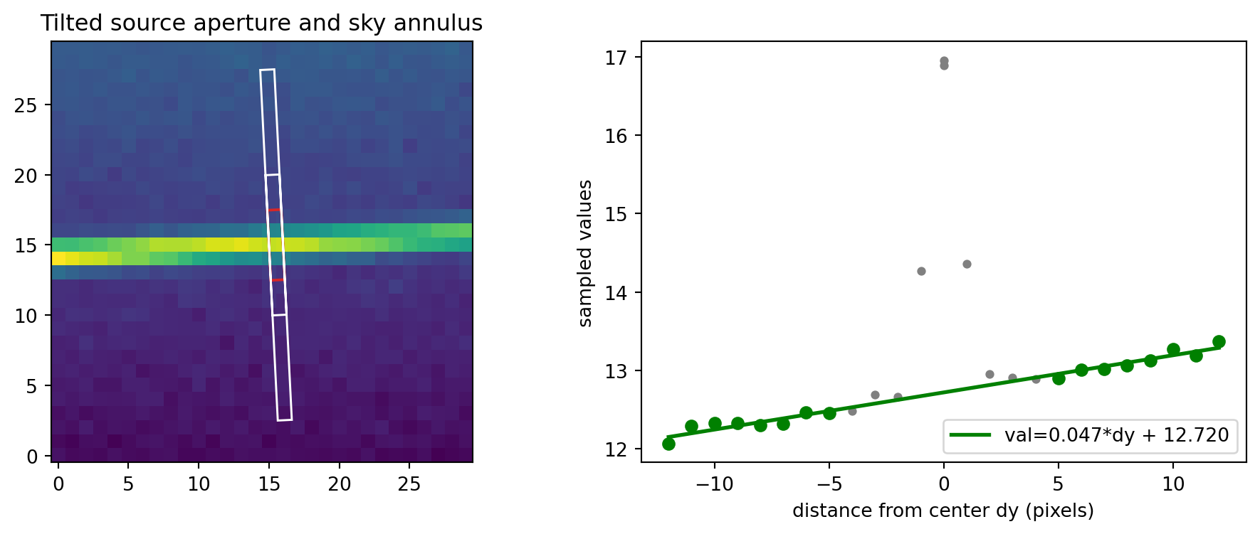

The annulus only selects pixels. The background model is your choice: a median, a clipped statistic, a polynomial, or a model tied to the observing setup.

Full sky subtraction

Repeat the same sky fit at each wavelength-bin center. RectAp requires finite sizes, so use an image-covering finite height for the full subtraction strip; this is the practical equivalent of a full-height aperture for this image.

lambda_x = np.arange(nx, dtype=np.float64) + 0.5
trace_y_at_x = ny // 2 + trace_slope * (lambda_x - x0)
full_height = 2.0 * np.hypot(nx, ny)
positions = list(zip(lambda_x, trace_y_at_x, strict=True))

kw_an = dict(w_in=1.0, h_in=10.0, w_out=1.0, h_out=25.0, theta_in=theta)
kw_full_ap = dict(w=1.0, h=full_height, theta=theta)
src_aps = aap.RectAp(positions, w=1., h=5., theta=theta)
sky_ans = aap.RectAn(positions, **kw_an)
full_aps = aap.RectAp(positions, **kw_full_ap)

sky_sub_sum = np.zeros_like(longslit_image, dtype=np.float64)
sky_sub_n = np.zeros_like(longslit_image, dtype=np.int16)
sky_models = []

sky_vals, sky_pix, sky_offsets = sky_ans.sampled_values(
    longslit_image,
    flat=True,
    return_pix=True,
)
sky_yy, _ = sky_pix
full_vals, full_pix, full_offsets = full_aps.sampled_values(
    longslit_image,
    flat=True,
    return_pix=True,
)
full_yy, full_xx = full_pix

for idx, (_x_cen, y_cen) in enumerate(full_aps.positions):
    sky_lo, sky_hi = sky_offsets[idx], sky_offsets[idx + 1]
    full_lo, full_hi = full_offsets[idx], full_offsets[idx + 1]

    sky_dy = sky_yy[sky_lo:sky_hi] - y_cen
    sky_fit = np.polyfit(sky_dy, sky_vals[sky_lo:sky_hi], deg=1)
    sky_models.append(sky_fit)

    yy_i = full_yy[full_lo:full_hi].astype(int)
    xx_i = full_xx[full_lo:full_hi].astype(int)
    full_dy = full_yy[full_lo:full_hi] - y_cen
    full_sky_sub = full_vals[full_lo:full_hi] - np.polyval(sky_fit, full_dy)

    np.add.at(sky_sub_sum, (yy_i, xx_i), full_sky_sub)
    np.add.at(sky_sub_n, (yy_i, xx_i), 1)

sky_sub_image = np.full_like(longslit_image, np.nan, dtype=np.float64)
covered = sky_sub_n > 0
sky_sub_image[covered] = sky_sub_sum[covered] / sky_sub_n[covered]
sky_models = np.asarray(sky_models)

assert np.all(sky_sub_n[:, 1:-1] > 0)
assert np.isfinite(sky_sub_image[covered]).all()

flux = src_aps.apsum_exact(
    np.nan_to_num(sky_sub_image, nan=0.0),
    return_npix=False,
)
expected_flux = src_aps.apsum_exact(trace_signal, return_npix=False)

assert flux.shape == lambda_x.shape
assert np.nanmax(np.abs(flux[1:-1] - expected_flux[1:-1])) < 0.5

fig, axes = plt.subplots(1, 2, figsize=(9.5, 3.8), constrained_layout=True)

im = axes[0].imshow(sky_sub_image, origin="lower", cmap="viridis")
src_aps.plot(ax=axes[0], color="tab:red", lw=0.6)
axes[0].set_title("Sky-subtracted full strips")
fig.colorbar(im, ax=axes[0], fraction=0.046, pad=0.04)

axes[1].plot(lambda_x, flux, marker="o", label="measured")
axes[1].plot(lambda_x, expected_flux, color="black", lw=1.5, label="input source")
axes[1].set_xlabel(r"$\lambda$ pixel")
axes[1].set_ylabel("source flux")
axes[1].legend()

plt.show()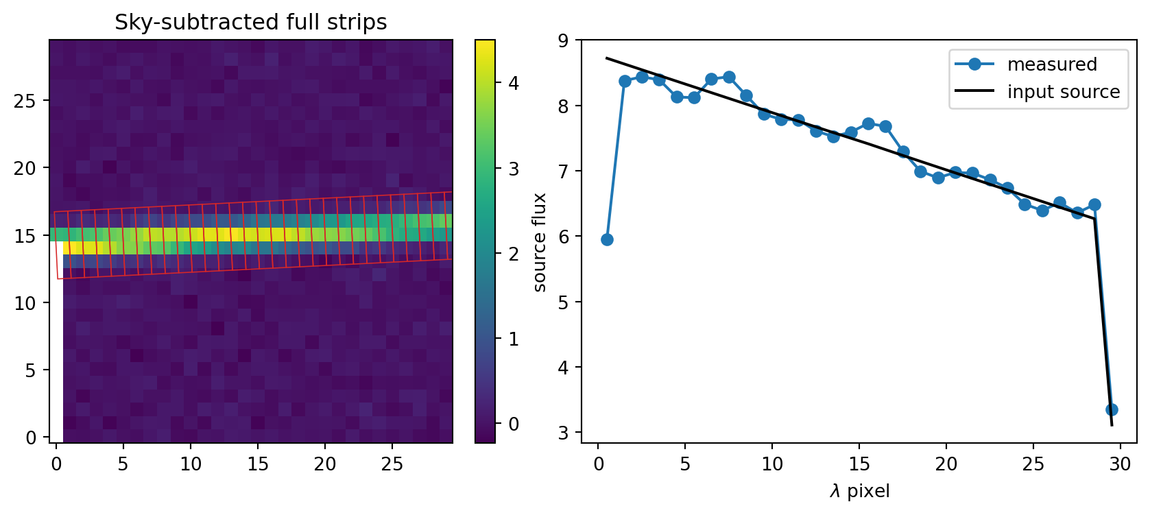

Elliptical inner boundary and circular outer boundary

The next example has an elliptical inner component and a circular coma:

• Large elliptical Gaussian coma
• Core circular Gaussian coma

Imagine we know the position angle and ellipticity of the inner coma component, but we want to subtract the circular outer coma to get the flux of inner component.

ny, nx = 90, 90
yy, xx = np.mgrid[:ny, :nx]
x0, y0 = 45.0, 44.0
theta_inner = np.deg2rad(45.0)

dx = xx - x0
dy = yy - y0
x_rot = dx * np.cos(theta_inner) + dy * np.sin(theta_inner)
y_rot = -dx * np.sin(theta_inner) + dy * np.cos(theta_inner)
radius = np.hypot(dx, dy)

elliptical_inner = 20.0 * np.exp(
    -0.5 * ((x_rot / 5.0) ** 2 + (y_rot / 8.0) ** 2)
)
circular_coma = 12.0 * np.exp(-0.5 * (radius / 10.0) ** 2)
coma_image = elliptical_inner + circular_coma

coma_annulus = aap.EllipAn(
    (x0, y0),
    a_in=10.0,
    b_in=16.0,
    a_out=30.0,
    b_out=30.0,
    theta_in=theta_inner,
    theta_out=0.0,
)

coma_values, coma_pix = coma_annulus.sampled_values(coma_image, return_pix=True)
coma_values = coma_values[0]
coma_y, coma_x = coma_pix[0]
coma_radius = np.hypot(coma_x - x0, coma_y - y0)

assert coma_values.size == coma_radius.size
assert coma_values.size > 0

def radial_coma_model(distance):
    return np.exp(np.polyval(log_coma_fit, distance**2))

valid = coma_values > 0.0
log_coma_fit = np.polyfit(coma_radius[valid] ** 2, np.log(coma_values[valid]), deg=1)

coma_model = radial_coma_model(radius)
residual = coma_image - coma_model
annulus_model_values = radial_coma_model(coma_radius)
annulus_residual_mad = np.median(np.abs(coma_values - annulus_model_values))
image_rms = np.sqrt(np.mean(coma_image**2))
residual_rms = np.sqrt(np.mean(residual**2))

assert annulus_residual_mad < 0.35
assert residual_rms < image_rms

fig, axes = plt.subplots(1, 2, figsize=(9.5, 3.8), constrained_layout=True)

axes[0].scatter(coma_radius, coma_values, s=14, alpha=0.25)
r_plot = np.linspace(0.0, 30.0, 200)
axes[0].plot(r_plot, radial_coma_model(r_plot), color="tab:red", lw=2, label="fit")
axes[0].set_xlabel("distance from center (pixels)")
axes[0].set_ylabel("pixel value")
axes[0].legend()

axes[1].imshow(coma_image, origin="lower", cmap="magma")
coma_annulus.plot(ax=axes[1], color="white", lw=1.2)
axes[1].set_title("Ellipse-to-circle annulus")

plt.show()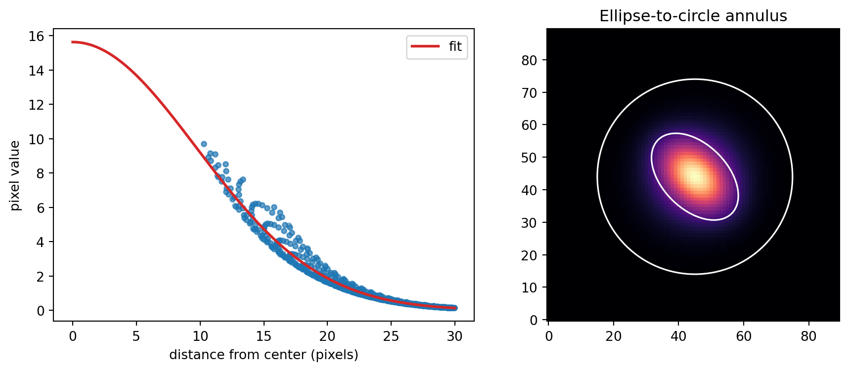

vmax = np.percentile(coma_image, 99.0)
residual_limit = np.percentile(np.abs(residual), 99.0)

fig, axes = plt.subplots(1, 3, figsize=(10.5, 3.5), constrained_layout=True)

panels = [
    (coma_image, "image", "magma", 0.0, vmax),
    (coma_model, "radial coma model", "magma", 0.0, vmax),
    (residual, "residual", "coolwarm", -residual_limit, residual_limit),
]

for ax, (image, title, cmap, vmin, vmax_panel) in zip(axes, panels):
    im = ax.imshow(image, origin="lower", cmap=cmap, vmin=vmin, vmax=vmax_panel)
    ax.set_title(title)
    ax.set_xticks([])
    ax.set_yticks([])
    fig.colorbar(im, ax=ax, fraction=0.046, pad=0.04)

plt.show()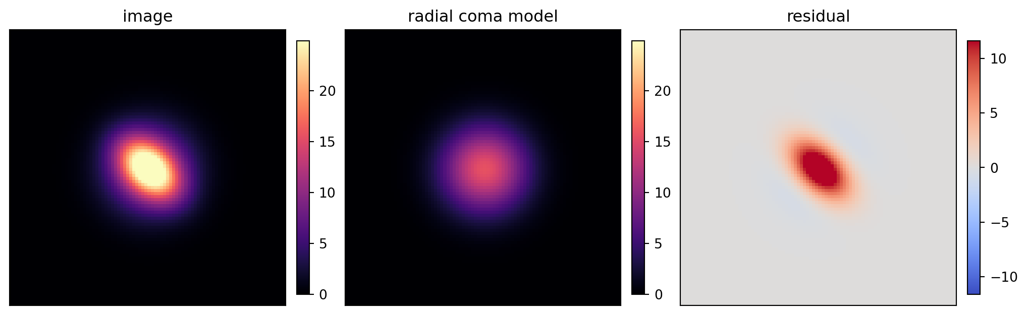

The model is intentionally simple. The radial fit removes most of the circular coma and leaves the non-circular inner component in the residual.

Maximum Performance

For mixed-shape annuli, the raw performance entry point is usually aapr.weights_*, because not every composite shape has a fused raw apsum_* function. The raw function returns flattened weights and integer bbox bounds. For more examples of raw call patterns, inspect astroapers.kernels.

import astroapers._rust as aapr

raw_coma = np.ascontiguousarray(coma_image, dtype=np.float64)
xpos = np.ascontiguousarray([x0], dtype=np.float64)
ypos = np.ascontiguousarray([y0], dtype=np.float64)

raw_weights, ixmins, ixmaxs, iymins, iymaxs = aapr.weights_ellip_ann_center(
    xpos,
    ypos,
    10.0,
    16.0,
    30.0,
    30.0,
    theta_inner,
    0.0,
)

raw_shape = (iymaxs[0] - iymins[0], ixmaxs[0] - ixmins[0])
raw_weights0 = np.asarray(raw_weights[0], dtype=np.float64).reshape(raw_shape)
raw_cutout = raw_coma[iymins[0]:iymaxs[0], ixmins[0]:ixmaxs[0]]
raw_values = raw_cutout[raw_weights0 > 0]

assert np.allclose(raw_values, coma_values)
raw_values.size, np.median(raw_values)

(2308, np.float64(0.9191297285514882))