import numpy as np
import matplotlib.pyplot as plt
import astroapers as aapAperture gallery
This page shows the built-in aperture and annulus families, then uses PathAp to illustrate custom apertures made from straight lines, circular arcs, and holes. All coordinates are pixel coordinates; angles are radians measured counterclockwise from the positive image x axis.
outline_center = (0.0, 0.0)
image_shape = (33, 33)
image_center = (16.0, 16.0)


def _style_outline_axis(ax, label, *, limit=8.0):
    ax.plot(*outline_center, marker="+", color="0.2", ms=7)
    ax.set_title(label)
    ax.set_aspect("equal")
    ax.set_xlim(-limit, limit)
    ax.set_ylim(-limit, limit)
    ax.set_xticks([])
    ax.set_yticks([])


def _show_mask(ax, make_ap, method, *, limit=8.0):
    ap = make_ap(image_center)
    weights = (ap.weights_exact() if method == "exact" else ap.weights_center())[0]
    bbox = ap.bboxes()[0]
    mask = bbox.to_image(weights, image_shape)
    assert mask.sum() > 0.0
    ny, nx = image_shape
    ax.imshow(
        mask,
        origin="lower",
        extent=(
            -image_center[0] - 0.5,
            nx - image_center[0] - 0.5,
            -image_center[1] - 0.5,
            ny - image_center[1] - 0.5,
        ),
        vmin=0.0,
        vmax=1.0,
        cmap="magma",
    )
    ax.set_title(f"{method}, npix={mask.sum():.1f}")
    ax.set_aspect("equal")
    ax.set_xlim(-limit, limit)
    ax.set_ylim(-limit, limit)
    ax.set_xticks([])
    ax.set_yticks([])
    return mask


def plot_shape_gallery(
    examples,
    *,
    color,
    limit=8.0,
    figsize=None,
    fill_outline=False,
):
    figsize = figsize or (2.6 * len(examples), 7.2)
    fig, axes = plt.subplots(
        3,
        len(examples),
        figsize=figsize,
        constrained_layout=True,
        squeeze=False,
    )
    for col, (label, make_ap) in enumerate(examples):
        outline = make_ap(outline_center)
        plot_kwargs = {"color": color, "lw": 2.0}
        if fill_outline:
            plot_kwargs.update(fill=True, alpha=0.25, edgecolor=color, facecolor=color)
        outline.plot(ax=axes[0, col], **plot_kwargs)
        _style_outline_axis(axes[0, col], label, limit=limit)

        exact = _show_mask(axes[1, col], make_ap, "exact", limit=limit)
        center = _show_mask(axes[2, col], make_ap, "center", limit=limit)
        assert exact.shape == center.shape == image_shape

    axes[0, 0].set_ylabel("outline")
    axes[1, 0].set_ylabel("exact")
    axes[2, 0].set_ylabel("center")
    return fig
Built-in aperture families
astroapers provides object classes for common circular, elliptical, rectangular, pill, and wedge aperture geometries. The same objects support plotting, bbox-tight weights, aperture sums, and effective pixel counts.
apertures = [
    ("CircAp", lambda c: aap.CircAp(c, r=4.0)),
    ("EllipAp", lambda c: aap.EllipAp(c, a=5.0, b=2.6, theta=np.deg2rad(25.0))),
    ("RectAp", lambda c: aap.RectAp(c, w=8.0, h=3.2, theta=np.deg2rad(-25.0))),
    (
        "PillAp",
        lambda c: aap.PillAp(c, w=5.0, a=2.5, b=1.4, theta=np.deg2rad(18.0)),
    ),
    (
        "WedgeAp",
        lambda c: aap.WedgeAp(
            c,
            r_in=1.5,
            r_out=6.0,
            theta_in=np.deg2rad(35.0),
            dtheta_in=np.deg2rad(85.0),
        ),
    ),
]

plot_shape_gallery(apertures, color="C0", limit=8.0, figsize=(13, 7.2))
plt.show()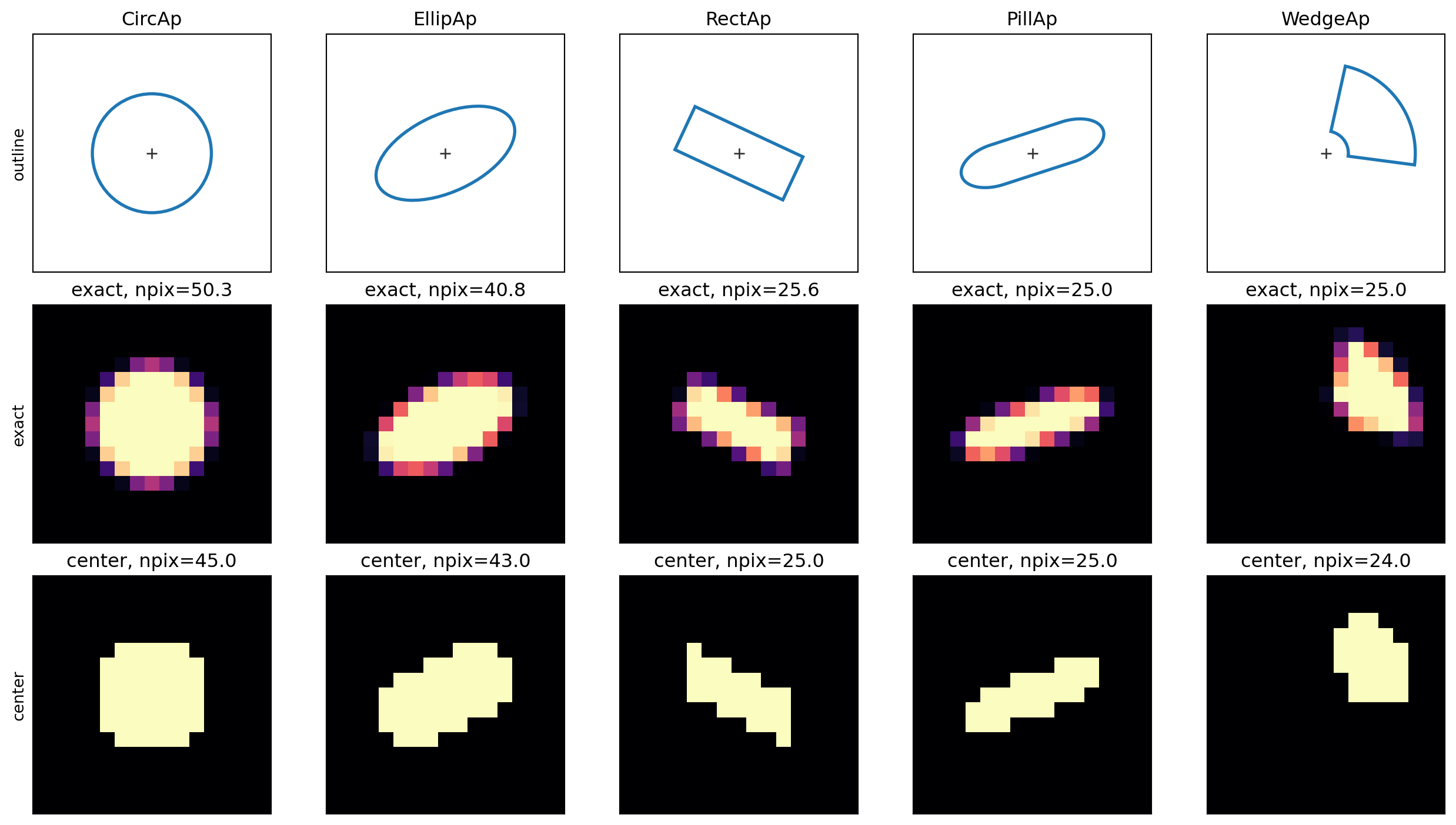
Annulus families with matched boundaries
Annulus classes expose the same measurement interface while subtracting an explicit inner shape from an outer shape. In the common case below, the inner and outer boundaries share the same center, orientation, and shape family.
matched_annuli = [
    ("CircAn", lambda c: aap.CircAn(c, r_in=2.0, r_out=5.4)),
    (
        "EllipAn",
        lambda c: aap.EllipAn(
            c,
            a_in=2.0,
            b_in=1.1,
            a_out=5.7,
            b_out=3.0,
            theta_in=np.deg2rad(25.0),
            theta_out=np.deg2rad(25.0),
        ),
    ),
    (
        "RectAn",
        lambda c: aap.RectAn(
            c,
            w_in=3.0,
            h_in=1.6,
            w_out=7.6,
            h_out=4.2,
            theta_in=np.deg2rad(-20.0),
            theta_out=np.deg2rad(-20.0),
        ),
    ),
    (
        "PillAn",
        lambda c: aap.PillAn(
            c,
            w_in=2.5,
            a_in=1.5,
            b_in=0.8,
            w_out=6.5,
            a_out=2.7,
            b_out=1.8,
            theta_in=np.deg2rad(18.0),
            theta_out=np.deg2rad(18.0),
        ),
    ),
]

plot_shape_gallery(
    matched_annuli,
    color="C3",
    limit=8.0,
    figsize=(11, 7.2),
    fill_outline=True,
)
plt.show()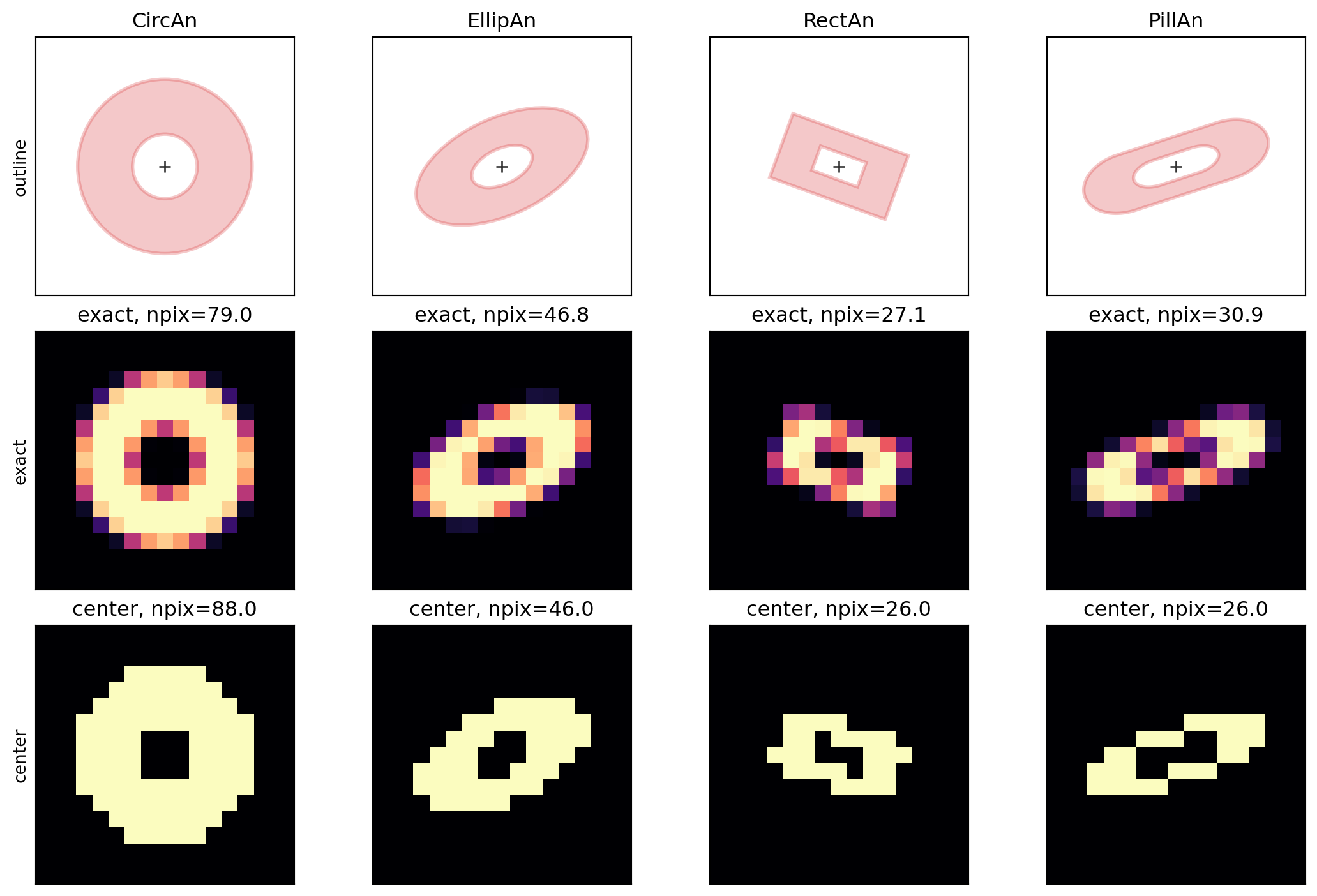
Annuli with independent inner and outer boundaries
Elliptical, rectangular, and pill annuli can use different inner and outer dimensions and rotations. This covers profile measurements where the fitted shape changes with radius.
split_annuli = [
    (
        "EllipAn",
        lambda c: aap.EllipAn(
            c,
            a_in=1.9,
            b_in=1.3,
            a_out=5.9,
            b_out=3.1,
            theta_in=np.deg2rad(-25.0),
            theta_out=np.deg2rad(30.0),
        ),
    ),
    (
        "RectAn",
        lambda c: aap.RectAn(
            c,
            w_in=2.8,
            h_in=1.7,
            w_out=7.8,
            h_out=4.5,
            theta_in=np.deg2rad(30.0),
            theta_out=np.deg2rad(-25.0),
        ),
    ),
    (
        "PillAn",
        lambda c: aap.PillAn(
            c,
            w_in=1.8,
            a_in=1.4,
            b_in=0.9,
            w_out=7.0,
            a_out=2.8,
            b_out=1.8,
            theta_in=np.deg2rad(-30.0),
            theta_out=np.deg2rad(25.0),
        ),
    ),
]

plot_shape_gallery(
    split_annuli,
    color="C4",
    limit=8.0,
    figsize=(8.5, 7.2),
    fill_outline=True,
)
plt.show()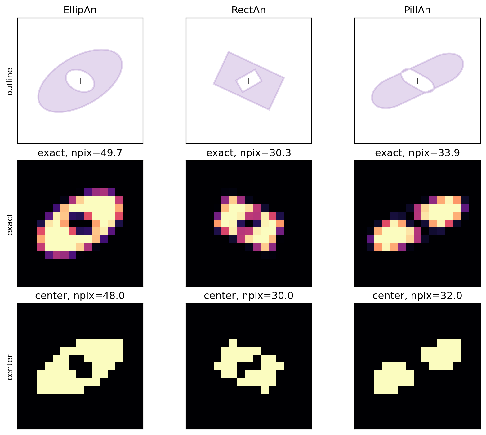
PathAp degrees of freedom
PathAp is for geometric apertures that do not fit the built-in families. Each closed path starts with ("move", x, y), continues with ("line", x, y) and ("arc", cx, cy, r, theta0, dtheta) commands, and ends with ("close",). Paths may also contain holes.
The path language is intentionally limited to straight line segments and circular arcs. Bezier curves, splines, elliptical arcs, Matplotlib paths, and Python callback masks are not supported. If another curve is flattened into line segments first, exact mode is exact for that flattened approximation.
rounded_lobe = [
    ("move", -7.0, -4.0),
    ("line", 0.5, -4.0),
    ("arc", 0.5, 0.0, 4.0, -0.5 * np.pi, np.pi),
    ("line", -7.0, 4.0),
    ("close",),
]

stepped = [
    ("move", -7.0, -5.0),
    ("line", -1.0, -5.0),
    ("line", -1.0, -2.0),
    ("line", 5.0, -2.0),
    ("line", 5.0, 3.0),
    ("line", 1.0, 3.0),
    ("line", 1.0, 6.0),
    ("line", -7.0, 6.0),
    ("close",),
]

outer_circle = [
    ("move", 7.0, 0.0),
    ("arc", 0.0, 0.0, 7.0, 0.0, 0.5 * np.pi),
    ("arc", 0.0, 0.0, 7.0, 0.5 * np.pi, 0.5 * np.pi),
    ("arc", 0.0, 0.0, 7.0, np.pi, 0.5 * np.pi),
    ("arc", 0.0, 0.0, 7.0, 1.5 * np.pi, 0.5 * np.pi),
    ("close",),
]
off_center_hole = [
    ("move", 4.4, 0.0),
    ("arc", 1.2, 0.0, 3.2, 0.0, 0.5 * np.pi),
    ("arc", 1.2, 0.0, 3.2, 0.5 * np.pi, 0.5 * np.pi),
    ("arc", 1.2, 0.0, 3.2, np.pi, 0.5 * np.pi),
    ("arc", 1.2, 0.0, 3.2, 1.5 * np.pi, 0.5 * np.pi),
    ("close",),
]

path_examples = [
    ("line + arc lobe", lambda c: aap.PathAp(c, rounded_lobe)),
    ("stepped polygon", lambda c: aap.PathAp(c, stepped)),
    ("path with hole", lambda c: aap.PathAp(c, outer_circle, holes=[off_center_hole])),
]

plot_shape_gallery(path_examples, color="C2", limit=8.0, figsize=(11, 7.2))
plt.show()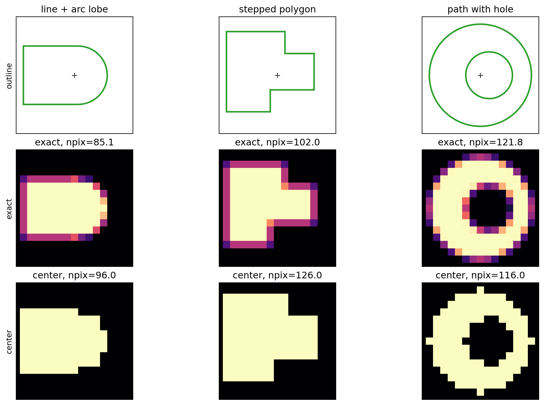
The mask rows show bbox-tight weights expanded back to an image grid. The same custom shapes can be evaluated at many centers, just like the built-in aperture classes.
positions = np.array(
    [
        [10.0, 10.0],
        [24.0, 16.0],
        [39.0, 10.0],
    ]
)
multi_path = aap.PathAp(positions, rounded_lobe)
test_image = np.ones((28, 50), dtype=float)
path_sums, path_npix = multi_path.apsum_exact(test_image)

fig, ax = plt.subplots(figsize=(7, 3.5))
ax.imshow(test_image, origin="lower", cmap="gray_r", vmin=0.0, vmax=1.0)
multi_path.plot(ax=ax, color="C2", lw=1.8)
ax.scatter(positions[:, 0], positions[:, 1], marker="+", color="0.2")
ax.set_title("One PathAp geometry at multiple centers")
plt.show()

np.column_stack([positions, path_sums, path_npix])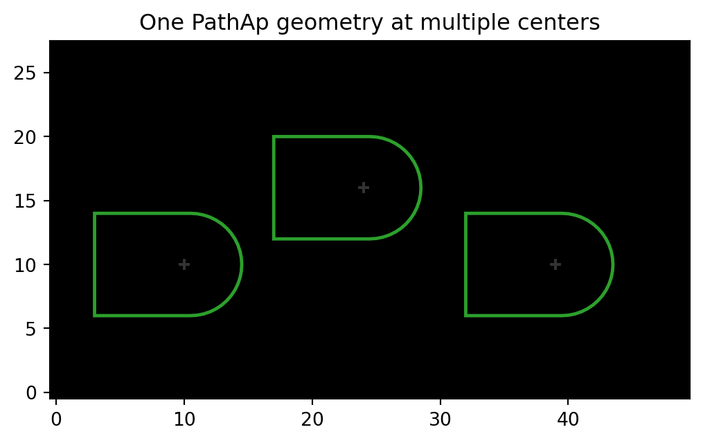
array([[10.        , 10.        , 85.13274123, 85.13274123],
       [24.        , 16.        , 85.13274123, 85.13274123],
       [39.        , 10.        , 85.13274123, 85.13274123]])