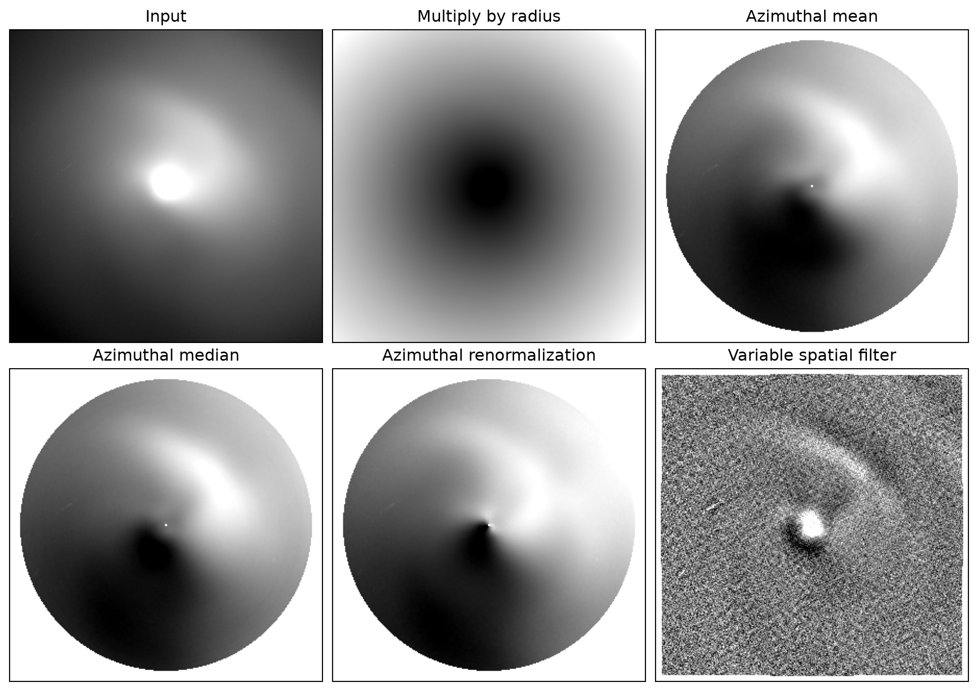
Apply five CometCIEF-style techniques and a direct annular variant to arrays and inspect a lossless FITS example.
Use air.viz.azimuthal_normalize to reveal variations around the nucleus. Keep the calibrated input for flux measurements: enhancement changes intensities and can create apparent structure around noise, stars, and masks.
The first five rows mirror the supplied CometCIEF techniques. The annular function is a direct radial-bin alternative to the polar azimuthal functions. The first technique defaults to a dust coma with a \(1/\rho\) profile; set power for another radial slope. Gas comae need not follow that default. Compare multiple techniques before interpreting a feature. Larson–Sekanina filtering is a separate difference method.
2. Load the packaged FITS example
Install astroimred[full] to run the plotting examples. The package includes the full 801 × 801 CometCIEF sample as a lossless xz archive. This example needs no download and does not write to the installed package.
import lzmafrom importlib.resources import as_file, filesimport astroimred as airimport matplotlib.pyplot as pltimport numpy as npfrom astropy.io import fitsresource = files("astroimred.viz").joinpath("data/CometCIEF_test.fits.xz")with as_file(resource) as path, lzma.open(path, "rb") as stream: image, header = fits.getdata(stream, header=True, memmap=False)assert image.shape == (801, 801)image.shape
(801, 801)
The source tutorial lists the nucleus at (400.5, 400.5) in one-based coordinates. AIR uses zero-based (x, y), so subtract one from both coordinates. Array indexing remains image[y, x].
center = (399.5, 399.5)
The tutorial calls the sample dust continuum, but its FITS header says OBJECT='HBcn'. The passband is unresolved. The examples demonstrate the algorithms; they do not establish which physical coma model fits this image.
3. Compare enhancements
Set the sampling
Option
Meaning
nrad
Polar radii from 1 through nrad pixels
ntheta
Number of equal-angle cells around each radius
subpixels=10
The source’s 10 × 10 midpoint sampling; larger values increase sampling resolution and cost
The values below are example settings. Choose radial coverage, angular resolution, rejection sigma, and kernel widths for your own image.
"mode" uses the MMM approximation 3 * median - 2 * mean, not a histogram mode. It can be zero, negative, or outside the retained sample range. Normalization accepts finite negative divisors; zero or nonfinite divisors are undefined. Renormalization requires a finite positive retained sample standard deviation.
Records the bins or polar cells used in one enhancement pass; performs no estimation
For a callable, pass a function that accepts one finite 1-D array of retained samples and returns one real scalar. Empty rings skip the callable, and a nonfinite result is undefined. Use this for custom estimators without new statistic-name aliases.
Choose clipping independently
Option
Meaning
sigma=None
Disable clipping
Scalar sigma or (lower, upper)
Symmetric or asymmetric thresholds
clip_center
"mean" or "median", independent of statistic
clip_scale
"std" (sample standard deviation, ddof=1) or "mad_std"
maxiters
Default 1: one pass. None: continue until no samples are rejected
Clipping changes the estimates, not the source samples that are transformed. For renormalization, clip_scale controls rejection only; the output always uses the retained sample standard deviation.
For example, a clipped MMM estimate with robust asymmetric rejection is selected by statistic="mode", sigma=(2, 3), maxiters=5, clip_center="median", clip_scale="mad_std". On a four-sample ring, sigma=3 with sample std can leave a bright outlier because that outlier inflates the same spread used for rejection. These settings define an estimator; they do not establish a physical coma model.
Each panel has its own display limits. Compare feature locations and shapes, not brightness between panels or between different radii of a normalized image.
Choose the radial profile power
power describes the assumed brightness law \(I\propto\rho^{\mathrm{power}}\), with radius in pixels. The correction uses the opposite exponent:
power
Correction averaged over each pixel’s midpoint grid
The factor is mean(rho**(-power)), not mean(rho)**(-power). Positive powers divide by radius: a midpoint exactly at \(\rho=0\) makes that pixel NaN. Grids that avoid zero can give finite but sampling-dependent values near the nucleus. This is a discrete midpoint average; for power >= 2, the continuous area integral diverges in pixels containing the nucleus. No radius floor is added. Nonfinite corrections and overflowed products become NaN; masks and nonfinite input pixels stay excluded.
Inspect the normalization statistics
Set return_stats=True to get an EnhancementResult: .image holds the enhanced array; .stats holds its NormStats record.
Field
Meaning
statistic, std
Retained-sample divisor/location and standard deviation (ddof=1)
n_valid, n_used
Support before and after sigma clipping
n_rejected
Sigma rejections only
n_samples
Polar: ntheta per ring. Annular: all in-frame pixel centers, including hard-masked and nonfinite centers
coverage
n_valid / n_samples; NaN when no in-frame samples exist
These describe estimation support, not propagated measurement uncertainty.
Exclude stars from estimates
statistic_mask excludes pixels from estimates while retaining their original finite values in the output. The existing mask remains a hard mask: it excludes pixels from both estimates and output. In a polar call, a masked midpoint excludes the whole polar cell from the estimate, while the original sample can still contribute to reconstruction.
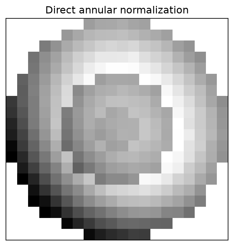
Direct annular normalization
Use annular_normalize when each original pixel should be divided by the statistic for the radial interval containing its pixel center. It accepts the same statistic and clipping options, but has no ntheta, subpixels, polar resampling, or reconstruction.
Intervals include the lower edge and exclude the upper edge: radii=[0, 2, 5, 10] means [0, 2), [2, 5), and [5, 10) pixels. There is no fractional area weighting. Pixels outside these intervals are NaN.
The example uses a compact source cut so those four edges cover most of the displayed image. The radius map and grouping are computed once per call; cache the returned result when changing only display settings. This tutorial makes no timing claim.
For example, an estimate-only mask removes a bright pixel from the annular mean while leaving its transformed value visible. No plotting is needed to inspect the normalization statistics:
For direct annuli, diagnostic.stats.radius is the midpoint of each supplied edge pair and diagnostic.stats.bin_edges preserves those exact edges. Polar rings use integer ring centers and have no bin_edges. Annular coverage is relative to in-frame centers, not a complete geometric annulus.
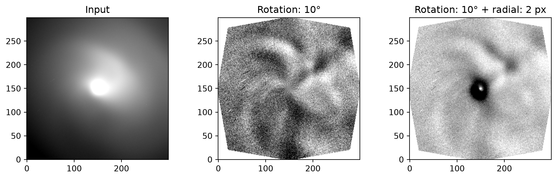
4. Apply Larson–Sekanina filtering
Use angle in degrees and radial_shift in pixels. The default radial_shift=0 subtracts two oppositely rotated samples. A positive shift samples inward; a negative shift samples outward.
The example shifts illustrate the controls; choose values for the scale of your features. With \(d_r\) in pixels and \(d_\theta\) in degrees, the original Larson & Sekanina (1984), equation (1) is
The two differences are summed, so angle=0 gives twice a radial difference. Changing the sign of angle leaves the result unchanged. No logarithm, background subtraction, or intensity normalization is applied.
Option or boundary
Behavior
interpolation="linear" (default)
Bilinear interpolation; smooths fine structure
interpolation="nearest"
Nearest pixel; half-integers round upward
Masked/nonfinite input or required sample
Output is NaN; zero-weight neighbors are ignored
Shifted position outside the pixel-center extent, or \(r-d_r<0\)
Output is NaN; no extrapolation
\(r=0\) with a nonzero radial shift
Output is NaN because the radial direction is undefined
Compare with the original image: centering errors and sharp features can produce positive/negative artifacts. Measure photometry on the original.
5. Handle masks and boundaries
Pass mask=True at pixels you want excluded. Masked arrays are also supported. Nonfinite inputs are excluded automatically. For a CCDData image, pass ccd.data and mask=ccd.mask explicitly.
Pixel centers outside the supplied intervals are NaN. Bounds include the lower edge and exclude the upper; there is no subpixel area weighting
Spatial filtering
Every neighbor must be available. A mask invalidates any output whose stencil touches it
Larson–Sekanina
Both shifted positions must be available; only nonzero-weight contributors affect validity
A contaminated or incomplete polar ring uses its remaining valid cells for the statistic. Partial azimuth coverage can bias the result.
For normalization, zero or nonfinite statistics, including a mode or callable result, yield NaN; finite negative divisors are retained. Renormalization requires finite location and positive retained sample variance. No small denominator is added, and no implicit background subtraction is performed.
For spatial filtering, log=True requires every unmasked finite pixel to be strictly positive. Otherwise it raises ValueError; it does not silently disable the logarithm.
Differences from the original programs
These are array implementations of the supplied techniques, with explicit undefined-data behavior. They are not bit-for-bit replicas of the Fortran programs.
Centers are zero-based, outputs are float64, and no whole-image mean is forced to 100. The original input is never modified.
Polar sampling retains equal-angle cells, nearest-pixel lookup, and configurable subpixel averaging. Negative values remain valid; no sentinel intensities or denominator floors are used.
Both polar normalizers support mean, median, the MMM mode approximation, and callables. sigma applies to every statistic; the default is one pass (maxiters=1), while maxiters=None iterates to convergence. clip_center and clip_scale control rejection independently of the selected statistic.
Renormalization defaults to the mean location but accepts the same statistics. It maps with \(0.5 + (I - L)/(2 N s)\), where \(L\) is the selected location, \(N\) is nsigma, and \(s\) is the retained sample standard deviation (ddof=1). clip_scale affects rejection only. Values outside 0–1 are preserved.
The variable filter retains all eight neighbors when the width rounds to zero, so a flat field still gives zero. Unavailable neighbors become NaN instead of producing bright borders.
Sources and sample integrity
The techniques originate from CometCIEF and the comparative study by Samarasinha and Larson (2014). Credit the facility as Samarasinha, N. H., Martin, M. P., and Larson, S. M. (2013), Cometary Coma Image Enhancement Facility.
The archived FITS occupies 1,511,444 bytes instead of 2,574,720 bytes. Every original FITS byte, including its header, is recoverable. The bundled astroimred/viz/data/README.md records the compression comparison, SHA-256, source attribution, and unresolved passband and data-license metadata.