Read and inspect a FITS image

Create a synthetic FITS file, load CCDData, and inspect a summary table.

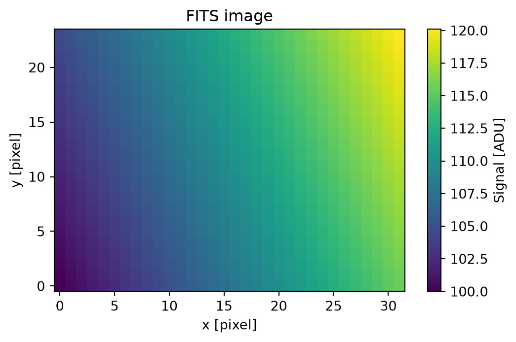
Run this example with astroimred[full]. It uses a temporary directory and synthetic data; it does not require telescope files or a network connection.

1. Create and read an image

from pathlib import Path
from tempfile import TemporaryDirectory

import numpy as np
from astropy.io import fits
from matplotlib import pyplot as plt

import astroimred as air

y, x = np.mgrid[:24, :32]
data = (100 + 0.5 * x + 0.2 * y).astype("float32")
header = fits.Header({"BUNIT": "adu", "OBJECT": "example", "EXPTIME": 30.0})

with TemporaryDirectory() as directory:
    path = Path(directory) / "example.fits"
    fits.writeto(path, data, header)
    ccd = air.load_ccd(path)
    summary = air.fits_summary([path], keywords=["OBJECT", "EXPTIME"])

np.testing.assert_array_equal(ccd.data, data)
ccd.shape, str(ccd.unit)

((24, 32), 'adu')

The returned CCDData keeps data, metadata, and units together. The temporary FITS file is removed after reading; ccd and summary remain available.

2. Inspect observation metadata

summary[["OBJECT", "EXPTIME"]]

	OBJECT	EXPTIME
0	example	30.0

For real observations, replace [path] with a list of FITS paths or a glob. Select header keywords explicitly to keep the table useful.

3. Display and bin pixels

fig, ax = plt.subplots(figsize=(6, 3.5), layout="constrained")
image = ax.imshow(ccd.data, origin="lower", cmap="viridis")
ax.set(xlabel="x [pixel]", ylabel="y [pixel]", title="FITS image")
fig.colorbar(image, ax=ax, label="Signal [ADU]")
plt.show()

binned = air.bin_ccd(ccd, factors=(2, 2))
assert binned.shape == (12, 16)
binned.shape

(12, 16)

factors uses (x, y) order for two-dimensional images. The default bin operation is the mean; use binfunc=np.sum when summed pixels are intended.

Continue with image combination, or look up fits_summary and load_ccd.